Introduction to Parallel Computing with R
The R Script associated with this page is available here. Download this file and open it (or copy-paste into a new script) with RStudio so you can follow along.
library(knitr)
library(raster)
library(rasterVis)
library(dplyr)
library(ggplot2)

## New Packages
library(foreach)
library(doParallel)
library(arm)
library(fields)
library(snow)
If you don’t have the packages above, install them in the package manager or by running install.packages("doParallel").
Simple examples
Sequential for() loop
x=vector()
for(i in 1:3)
  x[i]=i^2

x
## [1] 1 4 9Sequential foreach() loop
x <- foreach(i=1:3) %do%
  i^2

x
## [[1]]
## [1] 1
##
## [[2]]
## [1] 4
##
## [[3]]
## [1] 9Note that x is a list with one element for each iterator variable (i). You can also specify a function to use to combine the outputs with .combine. Let’s concatenate the results into a vector with c.
Sequential foreach() loop with .combine
x <- foreach(i=1:3,.combine='c') %do%
  i^2

x
## [1] 1 4 9Tells foreach() to first calculate each iteration, then .combine them with a c(...)
Sequential foreach() loop with .combine
x <- foreach(i=1:3,.combine='rbind') %do%
  i^2
x
## [,1]
## result.1 1
## result.2 4
## result.3 9Your turn
Write a foreach() loop that:
- generates 10 sets of 100 random values from a normal distribution (
rnorm()) - column-binds (
cbind) them.
x <- foreach(i=1:10,.combine='cbind') %do%
  rnorm(100)
head(x)%>%kable()| result.1 | result.2 | result.3 | result.4 | result.5 | result.6 | result.7 | result.8 | result.9 | result.10 |
|---|---|---|---|---|---|---|---|---|---|
| -0.0681918 | -1.4918930 | 1.0054695 | 0.5197490 | -0.1197721 | -1.2650029 | 0.3620914 | 0.3269817 | -1.0909711 | 0.9981671 |
| 0.9621697 | 0.1144240 | -0.7593140 | 0.6939953 | 0.4352010 | 0.4744220 | 0.5005153 | -0.3546572 | -0.5887028 | 0.7202042 |
| 0.2928529 | 0.6040765 | 0.4371090 | -0.2033832 | -0.3296048 | 0.3766330 | -0.2366459 | -0.0314536 | -0.4461361 | -0.5671695 |
| -0.9542502 | 0.2721461 | 0.3328846 | -1.3730961 | -0.6894935 | -0.2491623 | 0.7875628 | 1.6636158 | 0.4173346 | -1.3068274 |
| 1.4701807 | 0.0664254 | 1.2991707 | -0.7166465 | 1.8306685 | 2.1102283 | -0.1341981 | 0.1412985 | -1.7583039 | -0.6859997 |
| 2.4349876 | -1.8528417 | -0.0258563 | 1.9522308 | 0.3034693 | -0.2936645 | -0.6858021 | -1.0559328 | -0.1768820 | 0.8268803 |
dim(x)## [1] 100 10Parallel foreach() loop
So far we’ve only used %do% which only uses a single processor.
Before running foreach() in parallel, you have to register a parallel backend with one of the do functions such as doParallel(). On most multicore systems, the easiest backend is typically doParallel(). On linux and mac, it uses fork system call and on Windows machines it uses snow backend. The nice thing is it chooses automatically for the system.
# register specified number of workers
registerDoParallel(3)
# or, reserve all all available cores
#registerDoParallel()
# check how many cores (workers) are registered
getDoParWorkers()
## [1] 3NOTE It may be a good idea to use n-1 cores for processing (so you can still use your computer to do other things while the analysis is running)
To run in parallel, simply change the %do% to %dopar%. Wasn’t that easy?
## run the loop
x <- foreach(i=1:3, .combine='c') %dopar%
  i^2
x
## [1] 1 4 9A slightly more complicated example
In this section we will:
- Generate data with known parameters
- Fit a set of regression models using subsets of the complete dataset (e.g. bootstrapping)
- Compare processing times for sequential vs. parallel execution
For more on motivations to bootstrap, see here.
Make up some data:
n <- 100000              # number of data points
x1 <- rnorm (n)          # make up x1 covariate
b0 <- 1.8                # set intercept (beta0)
b1 <- -1.5                # set beta1
p = invlogit(b0+b1*x1)
y <- rbinom (n, 1, p)  # simulate data with noise
data=cbind.data.frame(y=y,x1=x1,p=p)
Let’s look at the data:
kable(head(data),row.names = F,digits = 2)| y | x1 | p |
|---|---|---|
| 0 | -0.26 | 0.90 |
| 1 | -0.53 | 0.93 |
| 1 | 0.34 | 0.78 |
| 1 | 1.37 | 0.44 |
| 1 | 0.18 | 0.82 |
| 1 | 0.64 | 0.70 |
ggplot(data,aes(y=x1,x=as.factor(y)))+
  geom_boxplot()+
  coord_flip()+
  geom_line(aes(x=p+1,y=x1),col="red",size=2,alpha=.5)+
  xlab("Binary Response")+
  ylab("Covariate")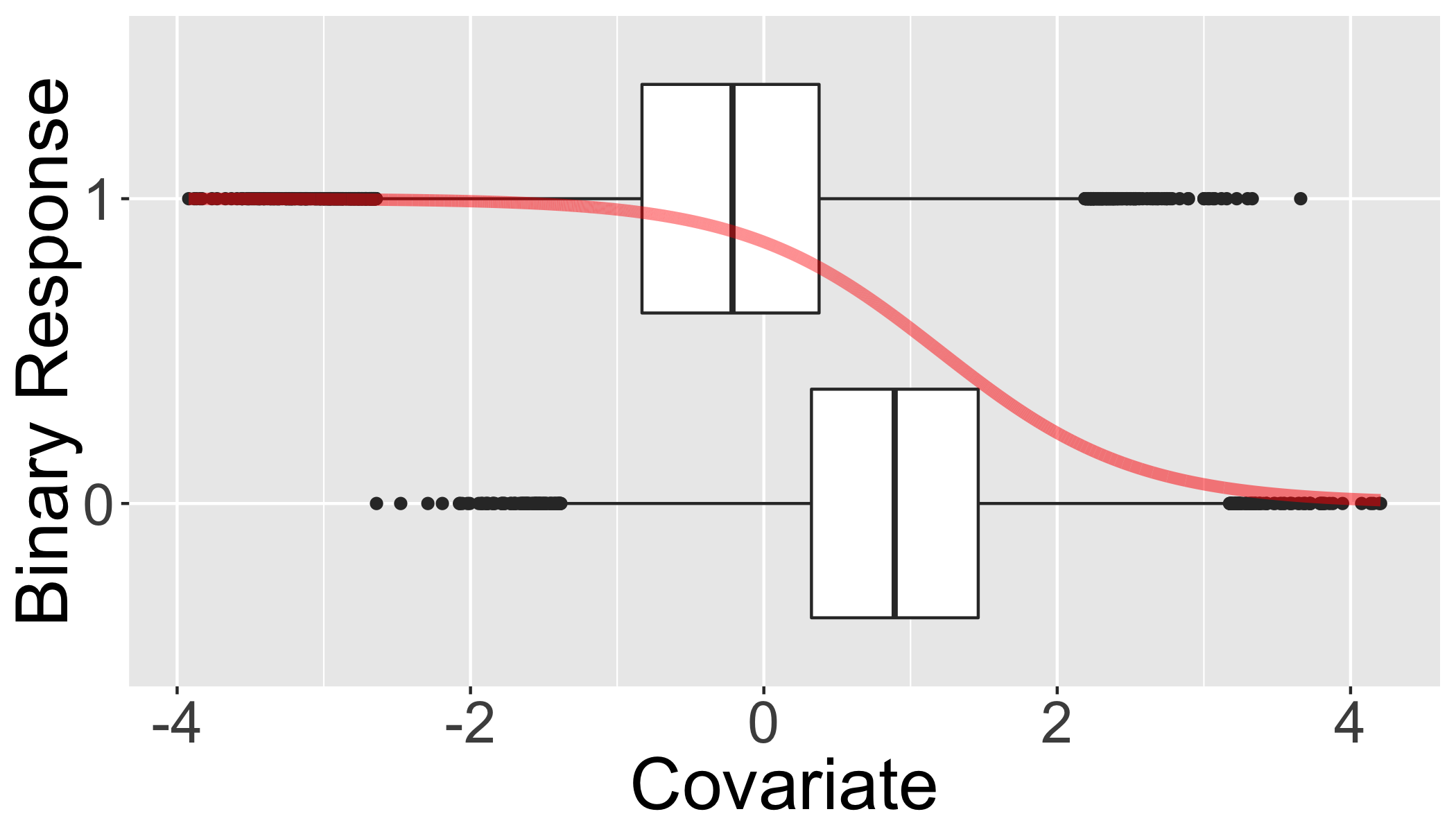
Sampling from a dataset with sample_n()
size=5
sample_n(data,size,replace=T)
## y x1 p
## 75062 0 0.7584076 0.6597968
## 84562 1 -1.2693708 0.9759683
## 92932 1 -0.1348258 0.8810319
## 77078 1 -0.1637584 0.8855061
## 45167 1 -1.7527452 0.9882155Simple Generalized Linear Model
This is the formal definition of the model we’ll use:
yi ∼ Bernoulli(pi)
logit(pi) = β0 + β1Xi
The index i identifies each grid cell (data point). β0 - β1 are model coefficients (intercept and slope), and yi is the simulated observation from cell i.
trials = 10000
tsize = 100

  ptime <- system.time({
  result <- foreach(i=1:trials,
                    .combine = rbind.data.frame) %dopar%
    {
      tdata=sample_n(data,tsize,replace=TRUE)
      M1=glm(y ~ x1, data=tdata, family=binomial(link="logit"))
      ## return parameter estimates
      cbind.data.frame(trial=i,t(coefficients(M1)))
    }
  })
ptime
## user system elapsed
## 30.551 3.218 35.485Look at results object containing slope and aspect from subsampled models. There is one row per sample (1:trials) with columns for the estimated intercept and slope for that sample.
kable(head(result),digits = 2)| trial | (Intercept) | x1 |
|---|---|---|
| 1 | 1.80 | -1.01 |
| 2 | 1.98 | -1.30 |
| 3 | 1.61 | -1.17 |
| 4 | 2.03 | -1.88 |
| 5 | 1.76 | -1.64 |
| 6 | 2.25 | -1.89 |
ggplot(dplyr::select(result,everything(),Intercept=contains("Intercept")))+
  geom_density(aes(x=Intercept),fill="black",alpha=.2)+
  geom_vline(aes(xintercept=b0),size=2)+
  geom_density(aes(x=x1),fill="red",alpha=.2)+
  geom_vline(aes(xintercept=b1),col="red",size=2)+
  xlim(c(-5,5))+
  ylab("Parameter Value")+
  xlab("Density")
## Warning: Removed 1 rows containing non-finite values (stat_density).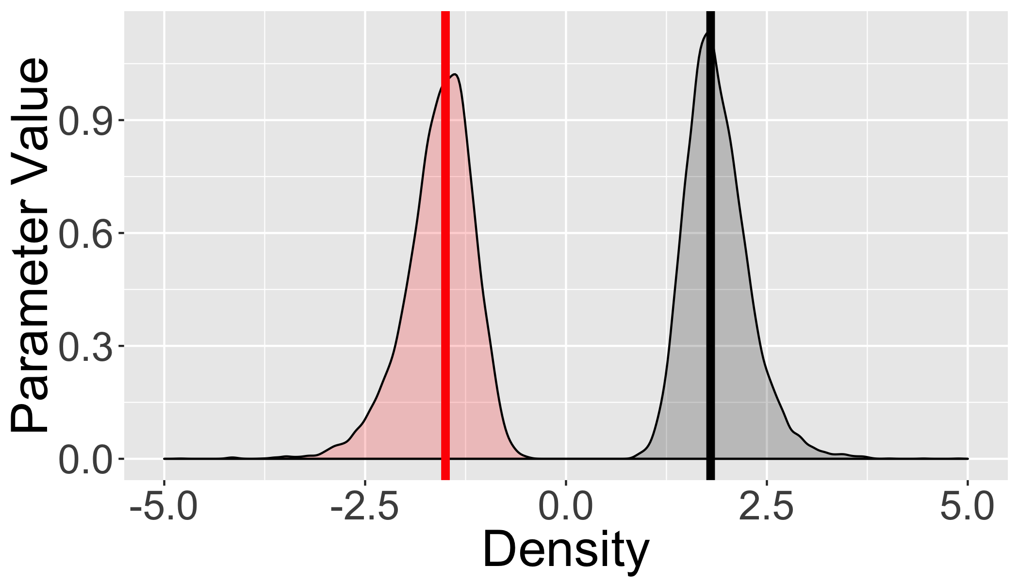
So we were able to perform 10^{4} separate model fits in 35.485 seconds. Let’s see how long it would have taken in sequence.
  stime <- system.time({
  result <- foreach(i=1:trials,
                    .combine = rbind.data.frame) %do%
    {
      tdata=sample_n(data,tsize,replace=TRUE)
      M1=glm(y ~ x1, data=tdata,family=binomial(link="logit"))
      ## return parameter estimates
      cbind.data.frame(trial=i,t(coefficients(M1)))
    }
  })
stime
## user system elapsed
## 33.835 2.533 37.473Your turn
- Generate some random as follows:
n <- 10000              # number of data points
x1 <- rnorm (n)          # make up x1 covariate
b0 <- 25                # set intercept (beta0)
b1 <- -15                # set beta1
y <- rnorm (n, b0+b1*x1,10)  # simulate data with noise
data2=cbind.data.frame(y=y,x1=x1)
Write a parallel foreach() loop that:
- selects a sample (as above) with
sample_n() - fits a ‘normal’ linear model with
lm() - Compiles the coefficient of determination (R^2) from each model
Hint: use summary(M1)$r.squared to extract the R^2 from model M1 (see ?summary.lm for more details).
trials = 100
tsize = 100

  result <- foreach(i=1:trials,.combine = rbind.data.frame) %dopar%
    {
      tdata=sample_n(data2,tsize,replace=TRUE)
      M1=lm(y ~ x1, data=tdata)
      cbind.data.frame(trial=i,
        t(coefficients(M1)),
        r2=summary(M1)$r.squared,
        aic=AIC(M1))
  }
Plot it:
ggplot(data2,aes(y=y,x=x1))+
  geom_point(col="grey")+
  geom_abline(data=dplyr::select(result,everything(),
                                 Intercept=contains("Intercept")),
              aes(intercept=Intercept,slope=x1),alpha=.5)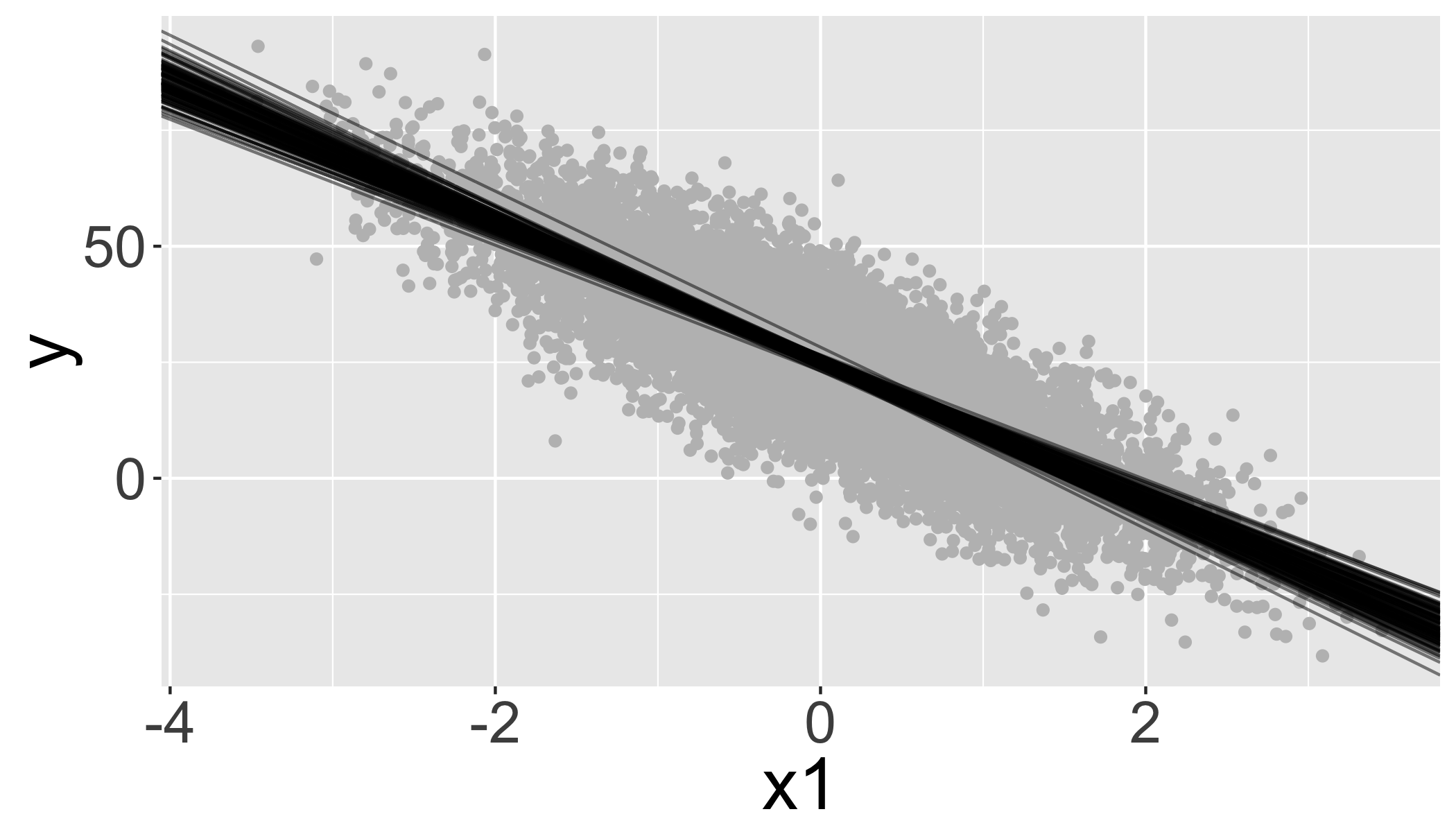
Writing data to disk
For long-running processes, you may want to consider writing results to disk as-you-go rather than waiting until the end in case of a problem (power failure, single job failure, etc.).
## assign target directory
td=tempdir()

  foreach(i=1:trials,
          .combine = rbind.data.frame) %dopar%
    {
      tdata=sample_n(data,
                     tsize,
                     replace=TRUE)
      M1=glm(y ~ x1,
             data=tdata,
             family=binomial(link="logit"))
      ## return parameter estimates
      results=cbind.data.frame(
      trial=i,
      t(coefficients(M1)))
      ## write results to disk
      file=paste0(td,"/results_",i,".csv")
      write.csv(results,file=file)
      return(NULL)
    }
## data frame with 0 columns and 0 rowsThat will save the result of each subprocess to disk (be careful about duplicated file names!):
list.files(td,pattern="results")%>%head()## [1] "results_1.csv" "results_10.csv" "results_100.csv" "results_11.csv"
## [5] "results_12.csv" "results_13.csv"Other useful foreach parameters
.inorder(true/false) results combined in the same order that they were submitted?.errorhandling(stop/remove/pass).packagespackages to made available to sub-processes.exportvariables to export to sub-processes
Spatial example
In this section we will:
- Generate some spatial data
- Tile the region to facilitate processing the data in parallel.
- Perform a moving window mean for the full area
- Compare processing times for sequential vs. parallel execution
Generate Spatial Data
A function to generate raster object with spatial autocorrelation.
simrast=function(nx=60,
                 ny=60,
                 theta=10,
                 seed=1234){
      ## create random raster with spatial structure
      ## Theta is scale of exponential decay
      ## This controls degree of autocorrelation,
      ## values ~1 are close to random while values ~nx/4 have high autocorrelation
     r=raster(nrows=ny, ncols=nx,vals=1,xmn=-nx/2,
              xmx=nx/2, ymn=-ny/2, ymx=ny/2)
      names(r)="z"
      # Simulate a Gaussian random field with an exponential covariance function
      set.seed(seed)  #set a seed so everyone's maps are the same
      grid=list(x=seq(xmin(r),xmax(r)-1,
                      by=res(r)[1]),
                y=seq(ymin(r),ymax(r)-1,res(r)[2]))
      obj<-Exp.image.cov(grid=grid,
                         theta=theta,
                         setup=TRUE)
      look<- sim.rf( obj)
      values(r)=t(look)*10
      return(r)
      }
Generate a raster using simrast.
r=simrast(nx=3000,ny=1000,theta = 100)
r
## class : RasterLayer
## dimensions : 1000, 3000, 3e+06 (nrow, ncol, ncell)
## resolution : 1, 1 (x, y)
## extent : -1500, 1500, -500, 500 (xmin, xmax, ymin, ymax)
## coord. ref. : NA
## data source : in memory
## names : z
## values : -47.03411, 40.15442 (min, max)Plot the raster showing the grid.
gplot(r)+
  geom_raster(aes(fill = value))+
  scale_fill_gradient(low = 'white', high = 'blue')+
  coord_equal()+ylab("Y")+xlab("X")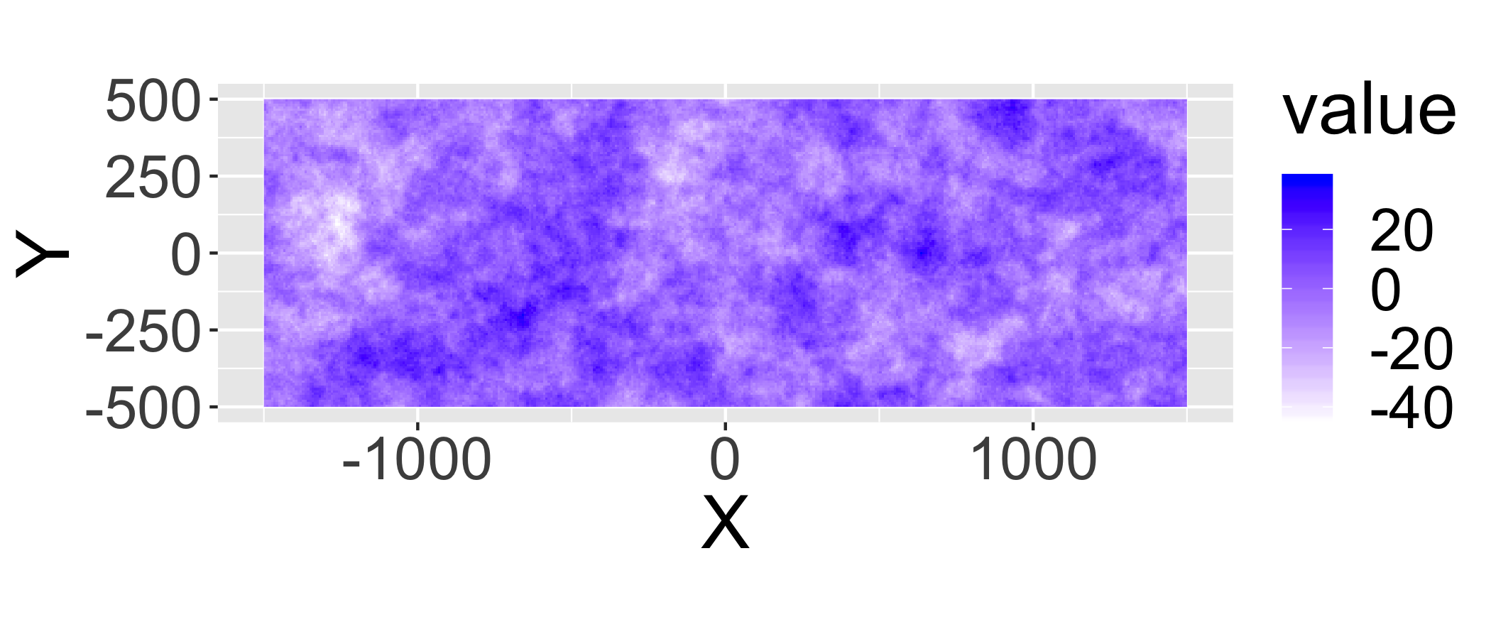
“Tile” the region
To parallelize spatial data, you often need to tile the data and process each tile separately. Here is a function that will take a bounding box, tile size and generate a tiling system. If given an overlap term, it will also add buffers to the tiles to reduce/eliminate edge effects, though this depends on what algorithm/model you are using.
tilebuilder=function(raster,size=10,overlap=NULL){
  ## get raster extents
  xmin=xmin(raster)
  xmax=xmax(raster)
  ymin=ymin(raster)
  ymax=ymax(raster)
  xmins=c(seq(xmin,xmax-size,by=size))
  ymins=c(seq(ymin,ymax-size,by=size))
  exts=expand.grid(xmin=xmins,ymin=ymins)
  exts$ymax=exts$ymin+size
  exts$xmax=exts$xmin+size
  if(!is.null(overlap)){
  #if overlapped tiles are requested, create new columns with buffered extents
    exts$yminb=exts$ymin
    exts$xminb=exts$xmin
    exts$ymaxb=exts$ymax
    exts$xmaxb=exts$xmax

    t1=(exts$ymin-overlap)>=ymin
    exts$yminb[t1]=exts$ymin[t1]-overlap
    t2=exts$xmin-overlap>=xmin
    exts$xminb[t2]=exts$xmin[t2]-overlap
    t3=exts$ymax+overlap<=ymax
    exts$ymaxb[t3]=exts$ymax[t3]+overlap
    t4=exts$xmax+overlap<=xmax
    exts$xmaxb[t4]=exts$xmax[t4]+overlap
  }
  exts$tile=1:nrow(exts)
  return(exts)
}
Generate a tiling system for that raster. Here will use only three tiles (feel free to play with this).
jobs=tilebuilder(r,size=1000,overlap=80)
kable(jobs,row.names = F,digits = 2)| xmin | ymin | ymax | xmax | yminb | xminb | ymaxb | xmaxb | tile |
|---|---|---|---|---|---|---|---|---|
| -1500 | -500 | 500 | -500 | -500 | -1500 | 500 | -420 | 1 |
| -500 | -500 | 500 | 500 | -500 | -580 | 500 | 580 | 2 |
| 500 | -500 | 500 | 1500 | -500 | 420 | 500 | 1500 | 3 |
Plot the raster showing the grid.
ggplot(jobs)+
  geom_raster(data=cbind.data.frame(
    coordinates(r),fill = values(r)),
    mapping = aes(x=x,y=y,fill = values(r)))+
  scale_fill_gradient(low = 'white', high = 'blue')+
  geom_rect(mapping=aes(xmin=xmin,xmax=xmax,
                        ymin=ymin,ymax=ymax),
            fill="transparent",lty="dashed",col="darkgreen")+
  geom_rect(aes(xmin=xminb,xmax=xmaxb,
                ymin=yminb,ymax=ymaxb),
            fill="transparent",col="black")+
  geom_text(aes(x=(xminb+xmax)/2,y=(yminb+ymax)/2,
                label=tile),size=10)+
  coord_equal()+ylab("Y")+xlab("X")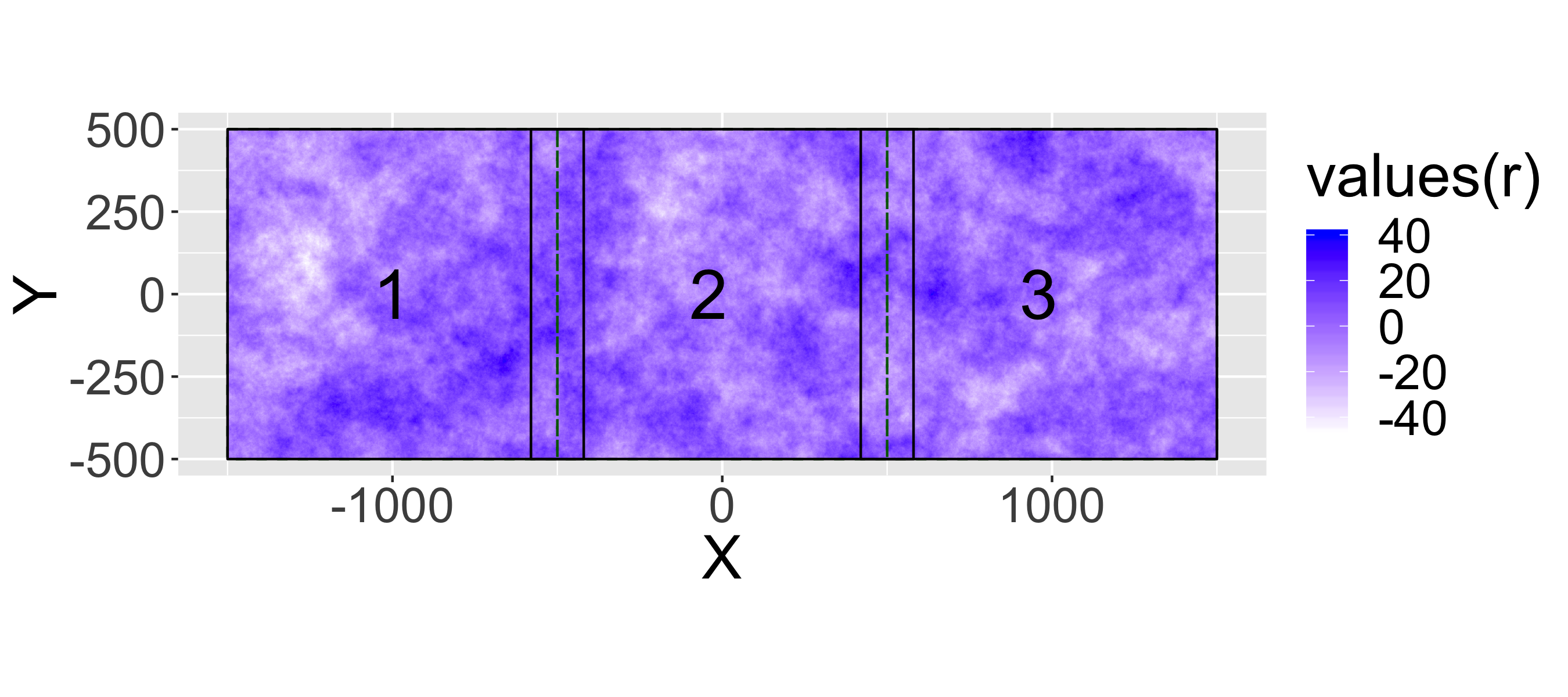
Run a simple spatial analysis: focal moving window
Use the focal function from the raster package to calculate a 3x3 moving window mean over the raster.
stime2=system.time({
  r_focal1=focal(r,w=matrix(1,101,101),mean,pad=T)
  })
stime2
## user system elapsed
## 38.885 0.594 42.513Plot it:
gplot(r_focal1)+
  geom_raster(aes(fill = value))+
  scale_fill_gradient(low = 'white', high = 'blue')+
  coord_equal()+ylab("Y")+xlab("X")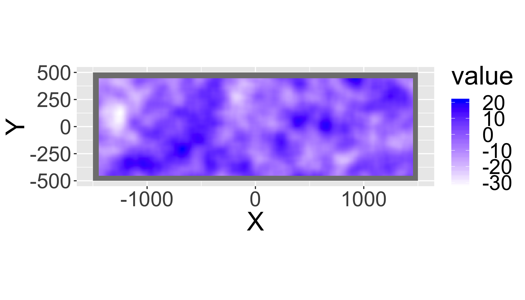
That works great (and pretty fast) for this little example, but as the data (or the size of the window) get larger, it can become prohibitive.
Repeat the analysis, but parallelize using the tile system.
First write a function that breaks up the original raster, computes the focal mean, then puts it back together. You could also put this directly in the foreach() loop.
focal_par=function(i,raster,jobs,w=matrix(1,101,101)){
  ## identify which row in jobs to process
  t_ext=jobs[i,]
  ## crop original raster to (buffered) tile
  r2=crop(raster,extent(t_ext$xminb,t_ext$xmaxb,
                        t_ext$yminb,t_ext$ymaxb))
  ## run moving window mean over tile
  rf=focal(r2,w=w,mean,pad=T)
  ## crop to tile
  rf2=crop(rf,extent(t_ext$xmin,t_ext$xmax,
                     t_ext$ymin,t_ext$ymax))
  ## return the object - could also write the file to disk and aggregate later outside of foreach()
  return(rf2)
}
Run the parallelized version.
registerDoParallel(3)

ptime2=system.time({
  r_focal=foreach(i=1:nrow(jobs),.combine=merge,
                  .packages=c("raster")) %dopar% focal_par(i,r,jobs)
  })
Are the outputs the same?
identical(r_focal,r_focal1)## [1] TRUESo we were able to process the data in 21.722 seconds when using 3 CPUs and 42.513 seconds on one CPU. That’s 2X faster for this simple example.
Parallelized Raster functions
Some functions in raster package also easy to parallelize.
ncores=2
beginCluster(ncores)

fn=function(x) x^3

system.time(fn(r))
## user system elapsed
## 0.123 0.003 0.128system.time(clusterR(r, fn, verbose=T))## user system elapsed
## 0.872 0.102 2.777endCluster()Does not work with:
- merge
- crop
- mosaic
- (dis)aggregate
- resample
- projectRaster
- focal
- distance
- buffer
- direction
High Performance Computers (HPC)
aka supercomputers, for example, check out the University at Buffalo HPC

Working on a cluster can be quite different from a laptop/workstation. The most important difference is the existence of scheduler that manages large numbers of individual tasks.
SLURM and R
You typically don’t run the script interactively, so you need to edit your script to ‘behave’ like a normal #! (linux command line) script. This is easy with getopt package.
cat(paste("
          library(getopt)
          ## get options
          opta <- getopt(
              matrix(c(
                  'date', 'd', 1, 'character'
              ), ncol=4, byrow=TRUE))
          ## extract value
          date=as.Date(opta$date)

          ## Now your script using date as an input
          print(date+1)
          q(\"no\")
          "
          ),file=paste("script.R",sep=""))
Then you can run this script from the command line like this:
Rscript script.R --date 2013-11-05You will need the complete path if Rscript is not on your system path. For example, on OS X, it might be at /Library/Frameworks/R.framework/Versions/3.2/Resources/Rscript.
Or even from within R like this:
system("Rscript script.R --date 2013-11-05")Driving cluster from R
Possible to drive the cluster from within R via SLURM. First, define the jobs and write that file to disk:
script="script.R"
dates=seq(as.Date("2000-01-01"),as.Date("2000-12-31"),by=60)
pjobs=data.frame(jobs=paste(script,"--date",dates))

write.table(pjobs,
  file="process.txt",
  row.names=F,col.names=F,quote=F)
This table has one row per task:
pjobs## jobs
## 1 script.R --date 2000-01-01
## 2 script.R --date 2000-03-01
## 3 script.R --date 2000-04-30
## 4 script.R --date 2000-06-29
## 5 script.R --date 2000-08-28
## 6 script.R --date 2000-10-27
## 7 script.R --date 2000-12-26Now identify other parameters for SLURM.
### Set up submission script
nodes=2
walltime=5
Write the SLURM script
### write SLURM script to disk from R

cat(paste("#!/bin/sh
#SBATCH --partition=general-compute
#SBATCH --time=00:",walltime,":00
#SBATCH --nodes=",nodes,"
#SBATCH --ntasks-per-node=8
#SBATCH --constraint=IB
#SBATCH --mem=300
# Memory per node specification is in MB. It is optional.
# The default limit is 3000MB per core.
#SBATCH --job-name=\"date_test\"
#SBATCH --output=date_test-srun.out
#SBATCH --mail-user=adamw@buffalo.edu
#SBATCH --mail-type=ALL
##SBATCH --requeue
#Specifies that the job will be requeued after a node failure.
#The default is that the job will not be requeued.

## Load necessary modules
module load openmpi/gcc-4.8.3/1.8.4
module load R

IDIR=~
WORKLIST=$IDIR/process.txt
EXE=Rscript
LOGSTDOUT=$IDIR/log/stdout
LOGSTDERR=$IDIR/log/stderr

### use mpiexec to parallelize across lines in process.txt
mpiexec -np $CORES xargs -a $WORKLIST -p $EXE 1> $LOGSTDOUT 2> $LOGSTDERR
",sep=""),file=paste("slurm_script.txt",sep=""))
Now we have a list of jobs and a qsub script that points at those jobs with the necessary PBS settings.
## run it!
system("sbatch slurm_script.txt")
## Check status with squeue
system("squeue -u adamw")
For more detailed information about the UB HPC, see the CCR Userguide.
Summary
Each task should involve computationally-intensive work. If the tasks are very small, it can take longer to run in parallel.
Choose your method
- Run from master process (e.g.
foreach)- easier to implement and collect results
- fragile (one failure can kill it and lose results)
- clumsy for big jobs
- Run as separate R processes
- see
getoptlibrary - safer for big jobs: each job completely independent
- update job list to re-run incomplete submissions
- compatible with slurm / cluster computing
- forces you to have a clean processing script
- see