The R Script associated with this page is available here. Download this file and open it (or copy-paste into a new script) with RStudio so you can follow along.

Summary

Access and work with station weather data from Global Historical Climate Network (GHCN)
Explore options for plotting timeseries
Trend analysis
Compute Climate Extremes

Climate Metrics

Climate Metrics: ClimdEX

Indices representing extreme aspects of climate derived from daily data:

alt text

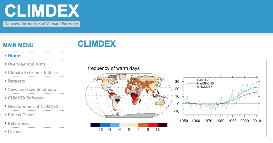
Climate Change Research Centre (CCRC) at University of New South Wales (UNSW) (climdex.org).

27 Core indices

For example:

FD Number of frost days: Annual count of days when TN (daily minimum temperature) < 0C.
SU Number of summer days: Annual count of days when TX (daily maximum temperature) > 25C.
ID Number of icing days: Annual count of days when TX (daily maximum temperature) < 0C.
TR Number of tropical nights: Annual count of days when TN (daily minimum temperature) > 20C.
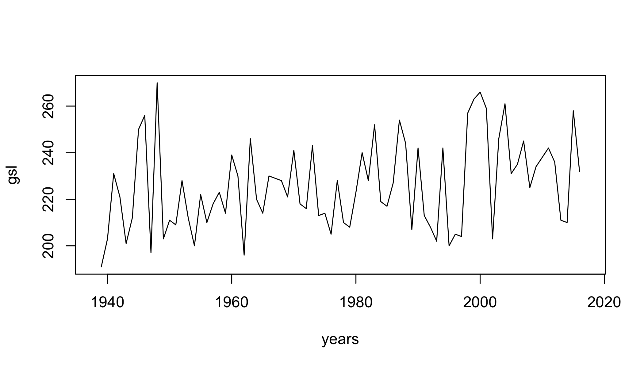
GSL Growing season length: Annual (1st Jan to 31st Dec in Northern Hemisphere (NH), 1st July to 30th June in Southern Hemisphere (SH)) count between first span of at least 6 days with daily mean temperature TG>5C and first span after July 1st (Jan 1st in SH) of 6 days with TG<5C.
TXx Monthly maximum value of daily maximum temperature
TN10p Percentage of days when TN < 10th percentile
Rx5day Monthly maximum consecutive 5-day precipitation
SDII Simple pricipitation intensity index

Weather Data

Climate Data Online

CDO

GHCN

ghcn

Options for downloading data

`FedData` package

National Elevation Dataset digital elevation models (1 and 1/3 arc-second; USGS)
National Hydrography Dataset (USGS)
Soil Survey Geographic (SSURGO) database
International Tree Ring Data Bank.
Global Historical Climatology Network (GHCN)

NOAA API

noaa api

National Climatic Data Center application programming interface (API).

`rNOAA` package

Handles downloading data directly from NOAA APIv2.

buoy_* NOAA Buoy data from the National Buoy Data Center
ghcnd_* GHCND daily data from NOAA
isd_* ISD/ISH data from NOAA
homr_* Historical Observing Metadata Repository
ncdc_* NOAA National Climatic Data Center (NCDC)
seaice Sea ice
storm_ Storms (IBTrACS)
swdi Severe Weather Data Inventory (SWDI)
tornadoes From the NOAA Storm Prediction Center

Libraries

library(raster)
library(sp)
library(rgdal)
library(ggplot2)
library(ggmap)
library(dplyr)
library(tidyr)
library(maps)
library(scales)
# New Packages
library(rnoaa)
library(climdex.pcic)
library(zoo)
library(reshape2)
library(broom)

Station locations

Download the GHCN station inventory with ghcnd_stations().

datadir="data"

st = ghcnd_stations()

## Optionally, save it to disk
# write.csv(st,file.path(datadir,"st.csv"))
## If internet fails, load the file from disk using:
# st=read.csv(file.path(datadir,"st.csv"))

GHCND Variables

5 core values:

PRCP Precipitation (tenths of mm)
SNOW Snowfall (mm)
SNWD Snow depth (mm)
TMAX Maximum temperature
TMIN Minimum temperature

And ~50 others! For example:

ACMC Average cloudiness midnight to midnight from 30-second ceilometer
AWND Average daily wind speed
FMTM Time of fastest mile or fastest 1-minute wind
MDSF Multiday snowfall total

`filter()` to temperature and precipitation

st=dplyr::filter(st,element%in%c("TMAX","TMIN","PRCP"))

Map GHCND stations

First, get a global country polygon

worldmap=map_data("world")

Plot all stations:

ggplot(data=st,aes(y=latitude,x=longitude)) +
  facet_grid(element~.)+
  annotation_map(map=worldmap,size=.1,fill="grey",colour="black")+
  geom_point(size=.1,col="red")+
  coord_equal()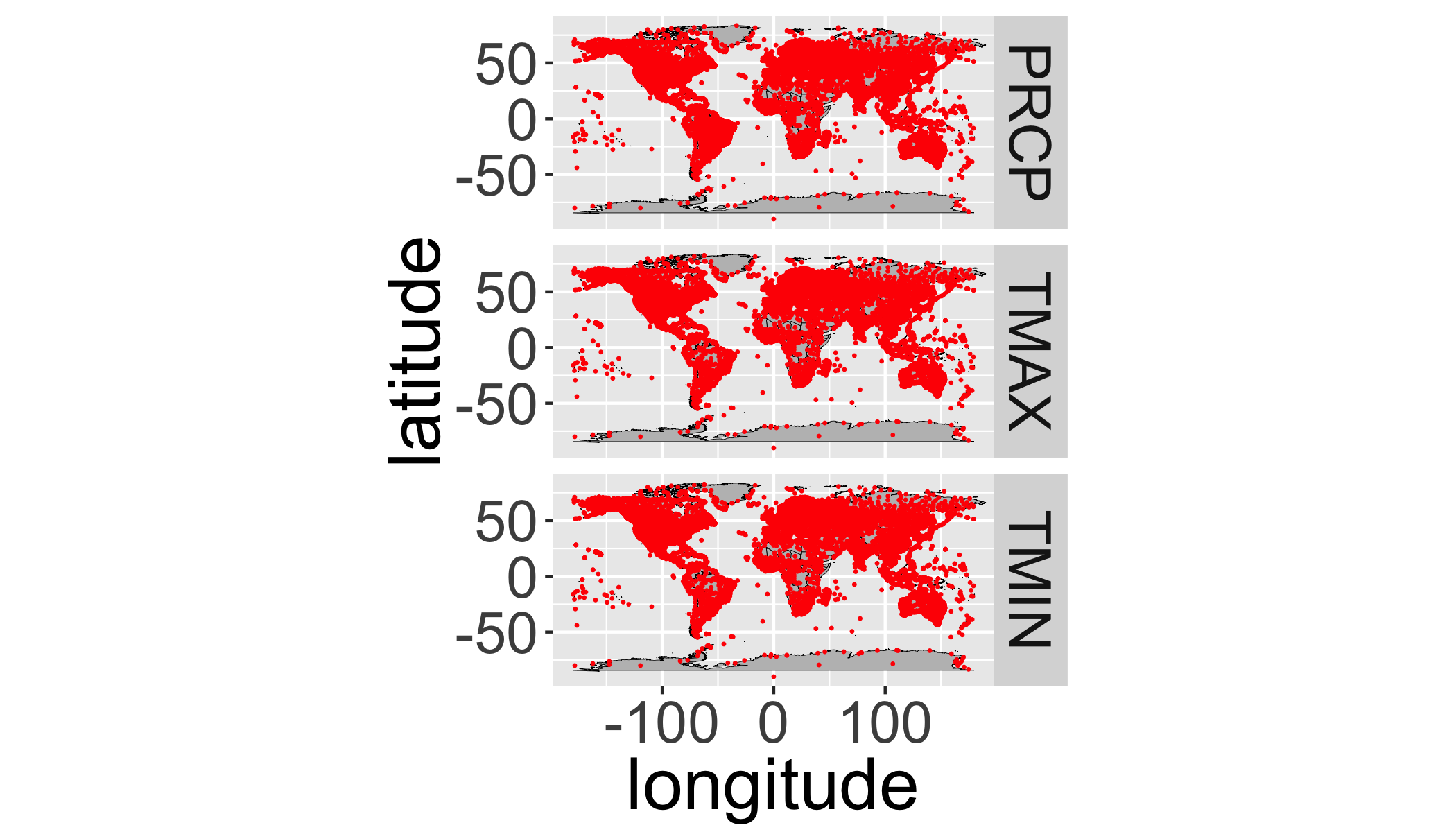

It’s hard to see all the points, let’s bin them…

ggplot(st,aes(y=latitude,x=longitude)) +
  annotation_map(map=worldmap,size=.1,fill="grey",colour="black")+
  facet_grid(element~.)+
  stat_bin2d(bins=100)+
  scale_fill_distiller(palette="YlOrRd",trans="log",direction=-1,
                       breaks = c(1,10,100,1000))+
  coord_equal()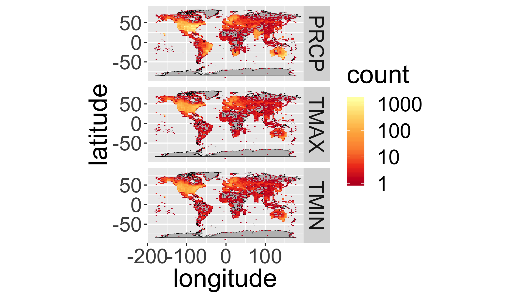

Your turn

Produce a binned map (like above) with the following modifications:

include only stations with a data record that starts before 1950 and ends after 2000 (keeping only complete records during that time).
include only tmax

ggplot(filter(st,
              first_year<=1950 & 
              last_year>=2000 & 
              element=="TMAX"),
       aes(y=latitude,x=longitude)) +
  annotation_map(map=worldmap,size=.1,fill="grey",colour="black")+
  stat_bin2d(bins=75)+
  scale_fill_distiller(palette="YlOrRd",trans="log",direction=-1,
    breaks = c(1,10,50))+
  coord_equal()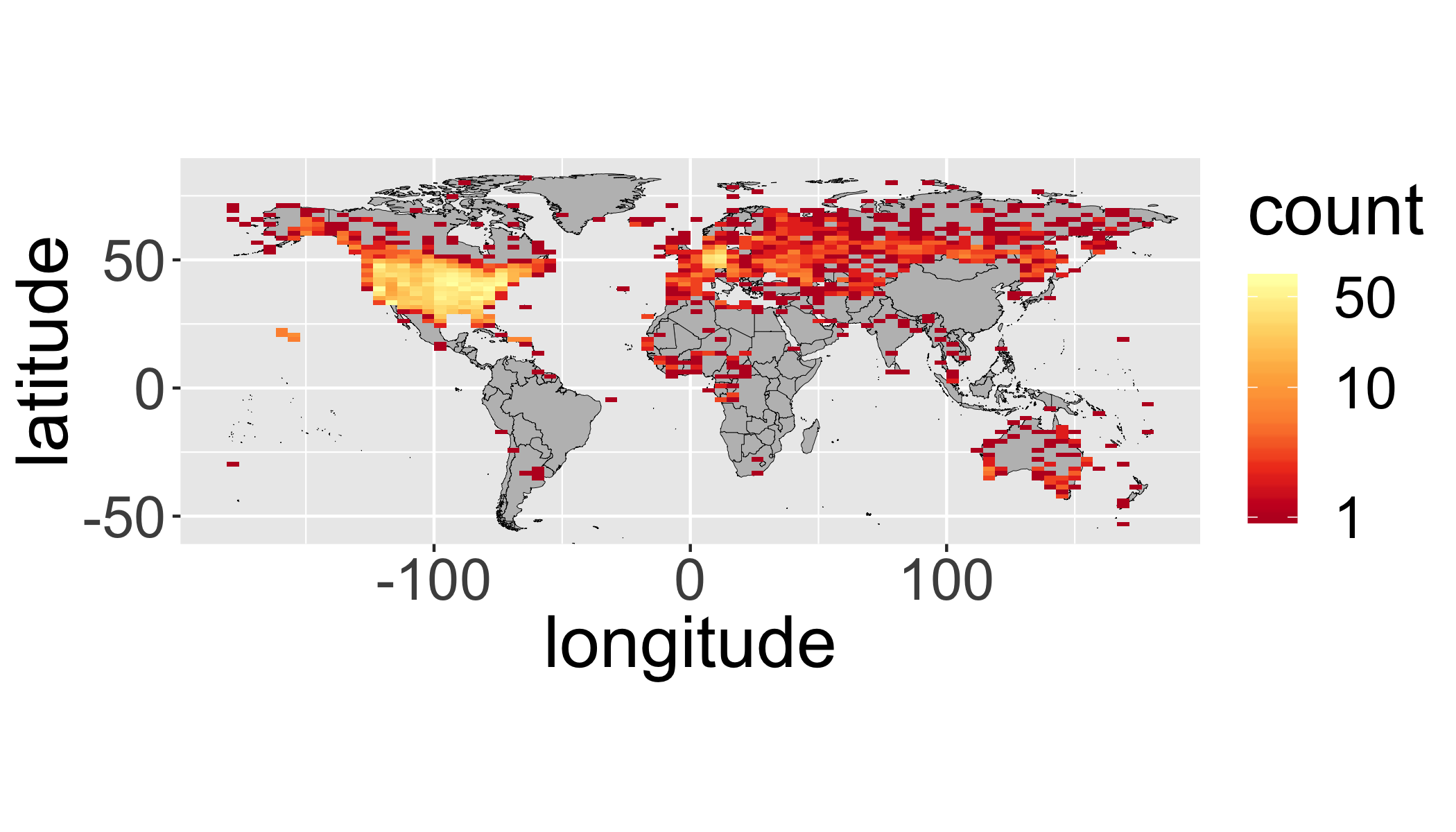

Download daily data from GHCN

ghcnd() will download a .dly file for a particular station. But how to choose?

`geocode` in ggmap package useful for geocoding place names

Geocodes a location (find latitude and longitude) using either (1) the Data Science Toolkit (http://www.datasciencetoolkit.org/about) or (2) Google Maps.

geocode("University at Buffalo, NY")

## Source : https://maps.googleapis.com/maps/api/geocode/json?address=University%20at%20Buffalo%2C%20NY

##         lon      lat
## 1 -78.78897 43.00081

However, you have to be careful:

geocode("My Grandma's house")

## Source : https://maps.googleapis.com/maps/api/geocode/json?address=My%20Grandma%27s%20house

##         lon      lat
## 1 -97.18744 32.82241

But this is pretty safe for well known places.

coords=as.matrix(geocode("Buffalo, NY"))

## Source : https://maps.googleapis.com/maps/api/geocode/json?address=Buffalo%2C%20NY

coords

##            lon      lat
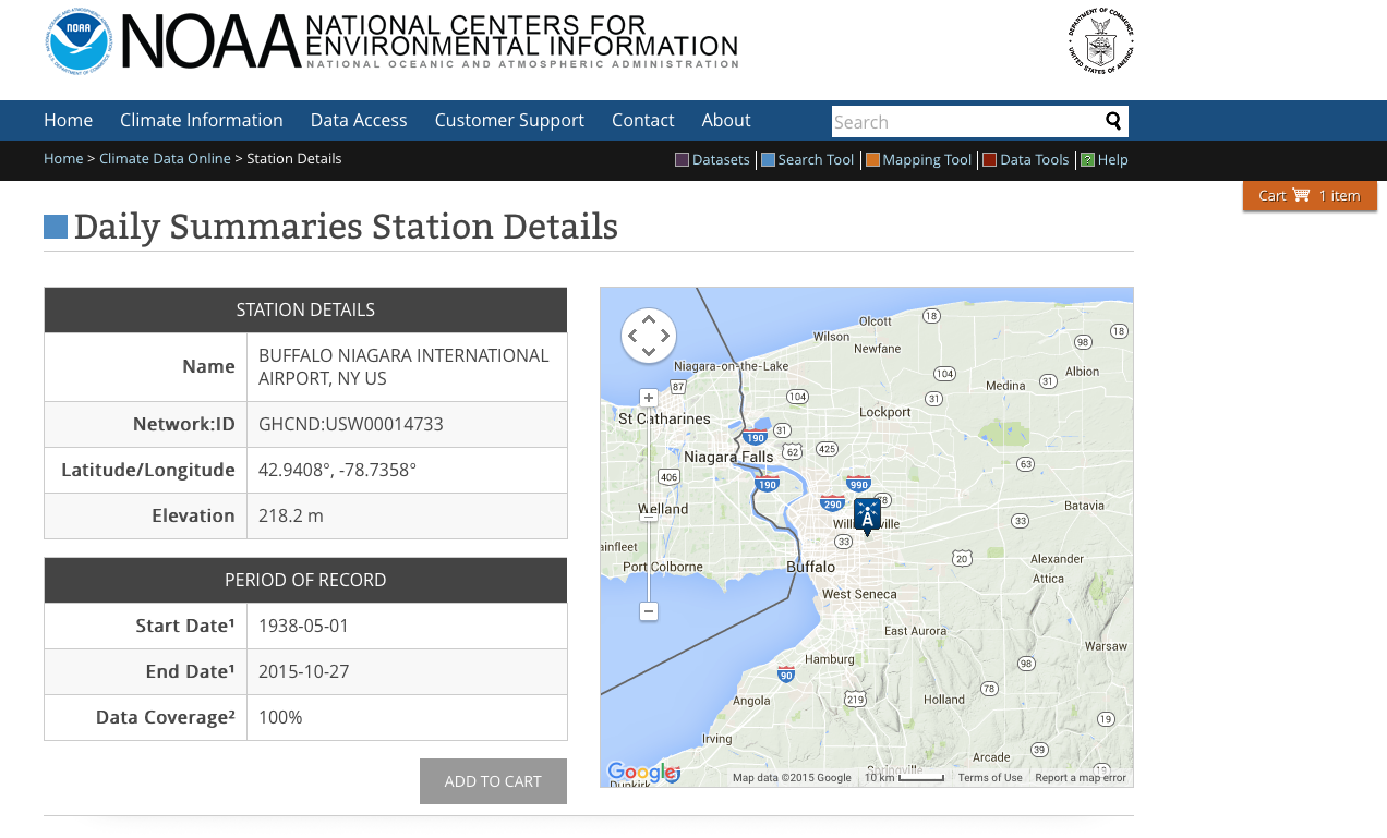
## [1,] -78.87837 42.88645

Now use that location to spatially filter stations with a rectangular box.

dplyr::filter(st,
              grepl("BUFFALO",name)&
              between(latitude,coords[2]-1,coords[2]+1) &
              between(longitude,coords[1]-1,coords[1]+1)&
         element=="TMAX")

## # A tibble: 3 x 11
##   id    latitude longitude elevation state name  gsn_flag wmo_id element
##   <chr>    <dbl>     <dbl>     <dbl> <chr> <chr> <chr>    <chr>  <chr>  
## 1 USC0…     42.9     -78.9    -1000. NY    BUFF… ""       ""     TMAX   
## 2 USC0…     42.9     -78.9      177. NY    BUFF… ""       ""     TMAX   
## 3 USW0…     42.9     -78.7      211. NY    BUFF… ""       HCN 7… TMAX   
## # ... with 2 more variables: first_year <int>, last_year <int>

You could also spatially filter using over() in sp package…

With the station ID, we can now download daily data from NOAA.

d=meteo_tidy_ghcnd("USW00014733",
                   var = c("TMAX","TMIN","PRCP"),
                   keep_flags=T)
head(d)

## # A tibble: 6 x 14
##   id    date       mflag_prcp mflag_tmax mflag_tmin  prcp qflag_prcp
##   <chr> <date>     <chr>      <chr>      <chr>      <dbl> <chr>     
## 1 USW0… 1938-05-01 T          " "        " "            0 " "       
## 2 USW0… 1938-05-02 T          " "        " "            0 " "       
## 3 USW0… 1938-05-03 " "        " "        " "           25 " "       
## 4 USW0… 1938-05-04 " "        " "        " "          112 " "       
## 5 USW0… 1938-05-05 T          " "        " "            0 " "       
## 6 USW0… 1938-05-06 " "        " "        " "           64 " "       
## # ... with 7 more variables: qflag_tmax <chr>, qflag_tmin <chr>,
## #   sflag_prcp <chr>, sflag_tmax <chr>, sflag_tmin <chr>, tmax <dbl>,
## #   tmin <dbl>

See CDO Daily Description and raw GHCND metadata for more details. If you want to download multiple stations at once, check out meteo_pull_monitors()

Quality Control: MFLAG

Measurement Flag/Attribute

Blank no measurement information applicable
B precipitation total formed from two twelve-hour totals
H represents highest or lowest hourly temperature (TMAX or TMIN) or average of hourly values (TAVG)
K converted from knots
…

See CDO Description

Quality Control: QFLAG

Blank did not fail any quality assurance check
D failed duplicate check
G failed gap check
K failed streak/frequent-value check
N failed naught check
O failed climatological outlier check
S failed spatial consistency check
T failed temporal consistency check
W temperature too warm for snow
…

See CDO Description

Quality Control: SFLAG

Indicates the source of the data…

Summarize QC flags

Summarize the QC flags. How many of which type are there? Should we be more conservative?

table(d$qflag_tmax)

## 
##           G     I 
## 29027     2    10

table(d$qflag_tmin)

## 
##           G     I     S 
## 29026     2     7     4

table(d$qflag_prcp)

## 
##           G 
## 29038     1

T failed temporal consistency check

Filter with QC data and change units

d_filtered=d%>%
  mutate(tmax=ifelse(qflag_tmax!=" "|tmax==-9999,NA,tmax/10))%>%  # convert to degrees C
  mutate(tmin=ifelse(qflag_tmin!=" "|tmin==-9999,NA,tmin/10))%>%  # convert to degrees C
  mutate(prcp=ifelse(qflag_tmin!=" "|prcp==-9999,NA,prcp))%>%  # convert to degrees C
  arrange(date)

Plot temperatures

ggplot(d_filtered,
       aes(y=tmax,x=date))+
  geom_line(col="red")

## Warning: Removed 11 rows containing missing values (geom_path).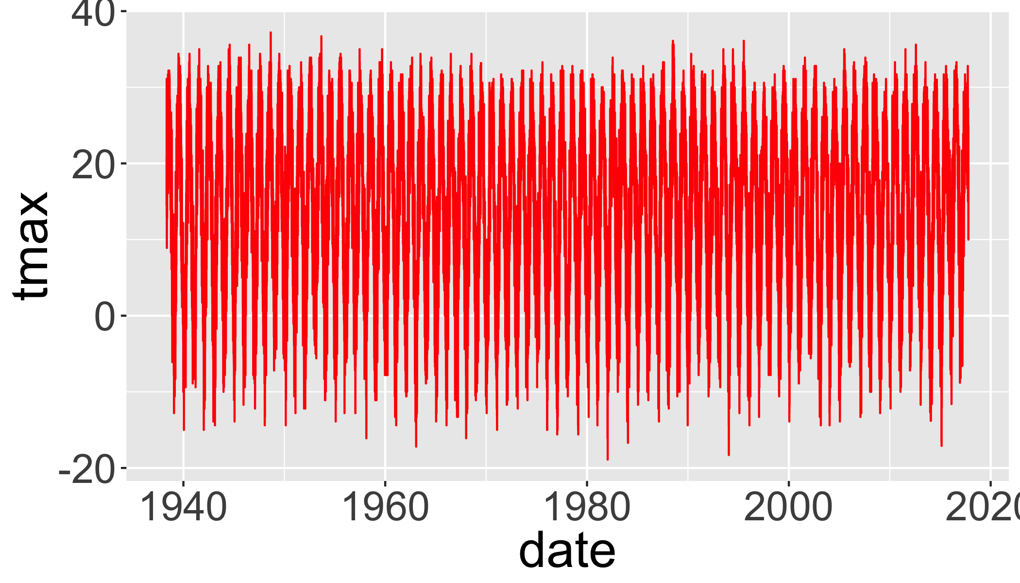

Limit to a few years and plot the daily range and average temperatures.

d_filtered_recent=filter(d_filtered,date>as.Date("2013-01-01"))

  ggplot(d_filtered_recent,
         aes(ymax=tmax,ymin=tmin,x=date))+
    geom_ribbon(col="grey",fill="grey")+
    geom_line(aes(y=(tmax+tmin)/2),col="red")

## Warning: Removed 11 rows containing missing values (geom_path).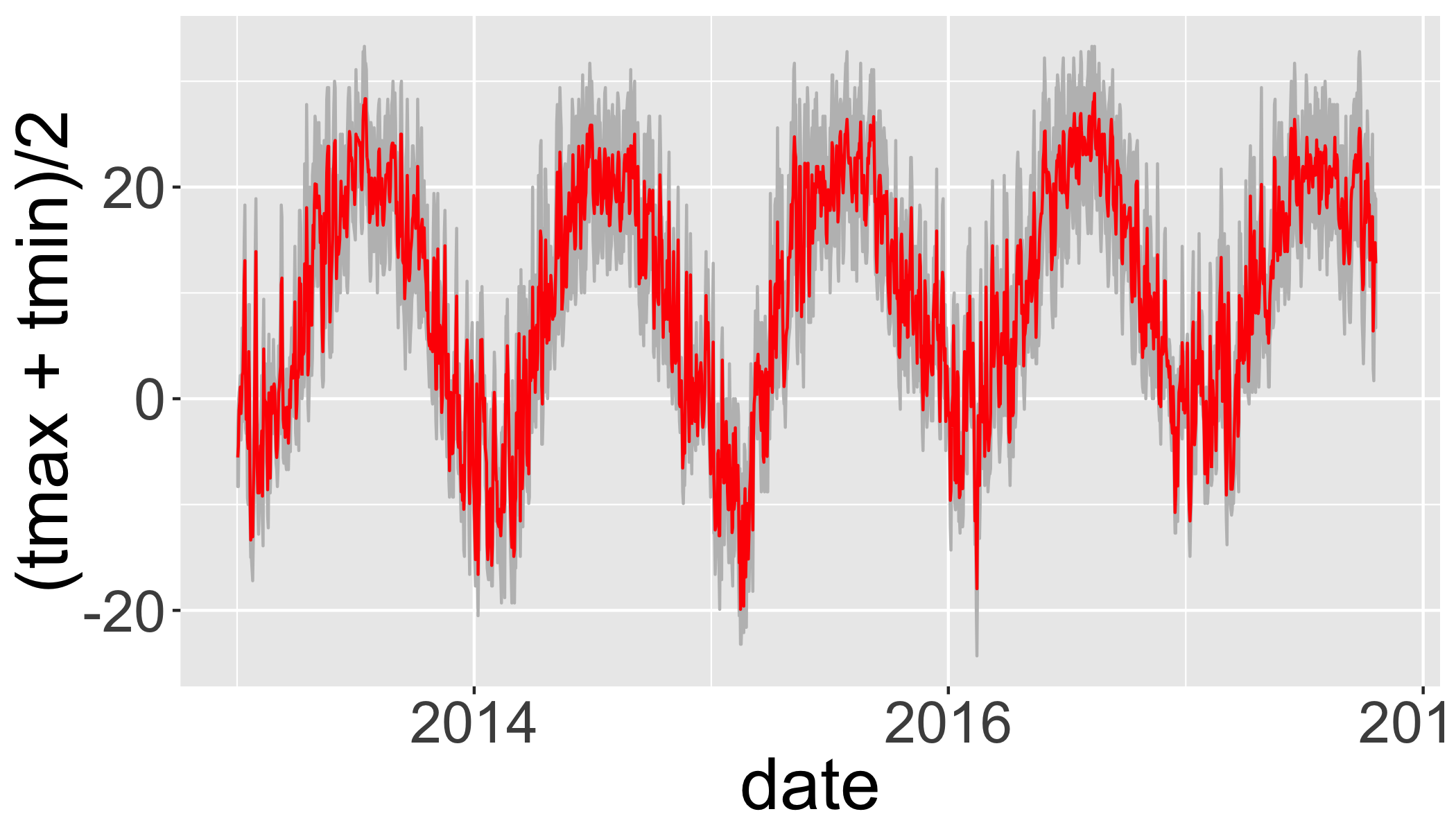

Zoo package for rolling functions

Infrastructure for Regular and Irregular Time Series (Z’s Ordered Observations)

rollmean(): Rolling mean
rollsum(): Rolling sum
rollapply(): Custom functions

Use rollmean to calculate a rolling 60-day average.

align whether the index of the result should be left- or right-aligned or centered

d_rollmean = d_filtered_recent %>% 
  arrange(date) %>%
  mutate(tmax.60 = rollmean(x = tmax, 60, align = "center", fill = NA),
         tmax.b60 = rollmean(x = tmax, 60, align = "right", fill = NA))

d_rollmean%>%
  ggplot(aes(ymax=tmax,ymin=tmin,x=date))+
    geom_ribbon(fill="grey")+
    geom_line(aes(y=(tmin+tmax)/2),col=grey(0.4),size=.5)+
    geom_line(aes(y=tmax.60),col="red")+
    geom_line(aes(y=tmax.b60),col="darkred")

## Warning: Removed 11 rows containing missing values (geom_path).

## Warning: Removed 70 rows containing missing values (geom_path).

## Warning: Removed 70 rows containing missing values (geom_path).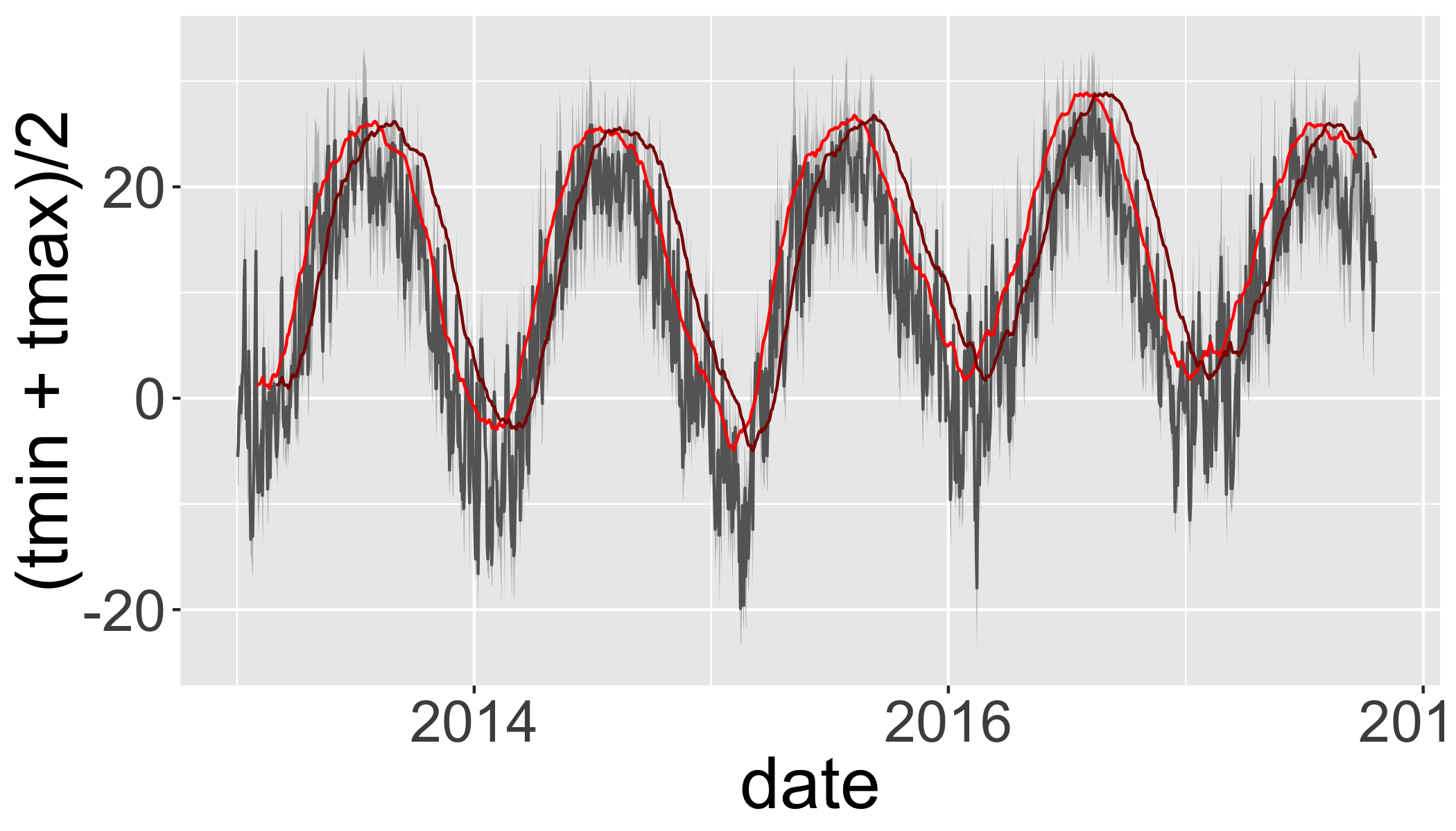

Your Turn

Plot a 30-day rolling “right” aligned sum of precipitation.

tp=d_filtered_recent %>%
  arrange(date)  %>% 
  mutate(prcp.30 = rollsum(x = prcp, 30, align = "right", fill = NA))

ggplot(tp,aes(y=prcp,x=date))+
  geom_line(aes(y=prcp.30),col="black")+ 
  geom_line(col="red")

## Warning: Removed 40 rows containing missing values (geom_path).

## Warning: Removed 11 rows containing missing values (geom_path).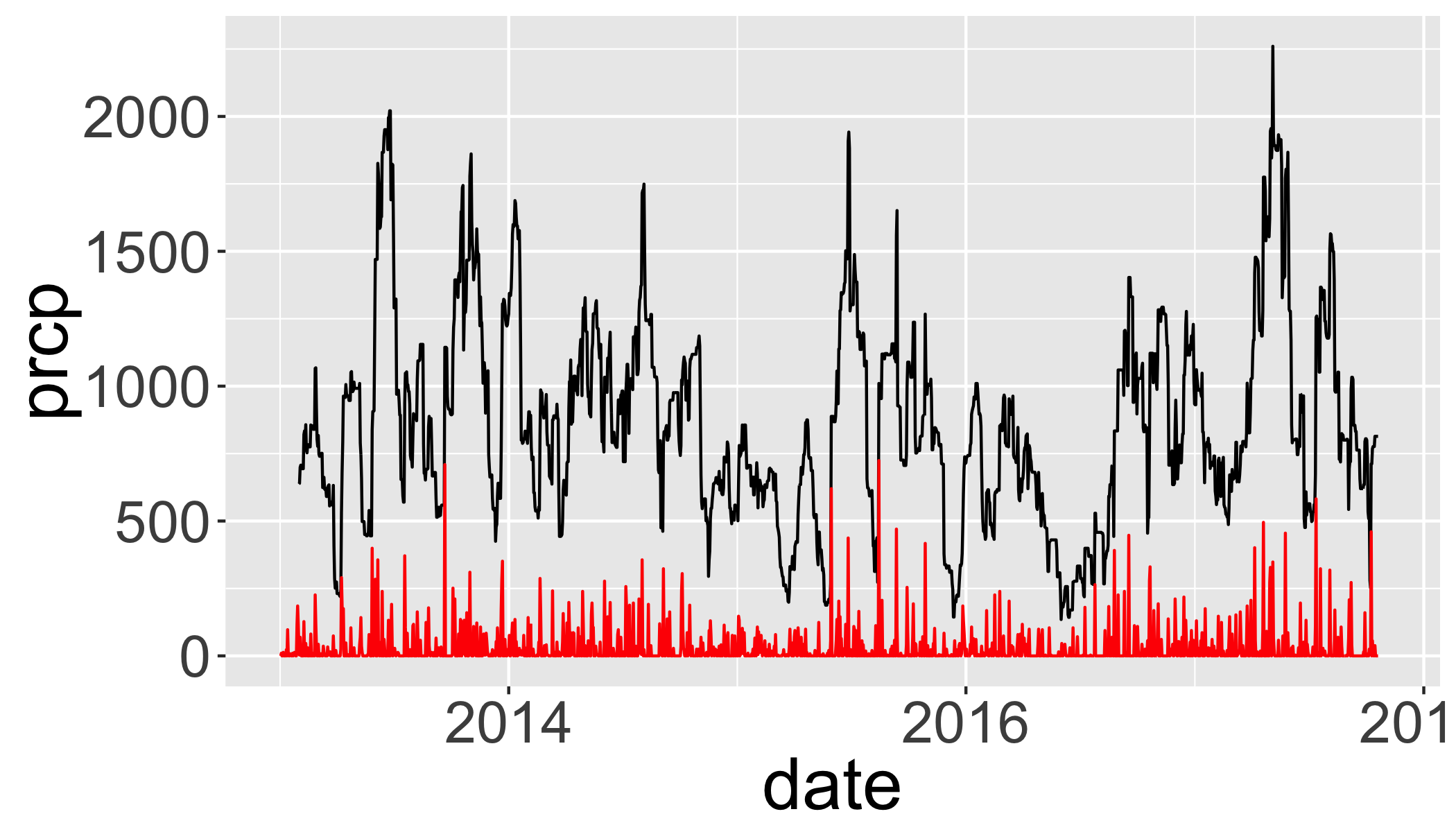

Time Series analysis

Most timeseries functions use the time series class (ts)

tmin.ts=ts(d_filtered_recent$tmin,frequency = 365)

Temporal autocorrelation

Values are highly correlated!

ggplot(d_filtered_recent,aes(y=tmin,x=lag(tmin)))+
  geom_point()+
  geom_abline(intercept=0, slope=1)

## Warning: Removed 12 rows containing missing values (geom_point).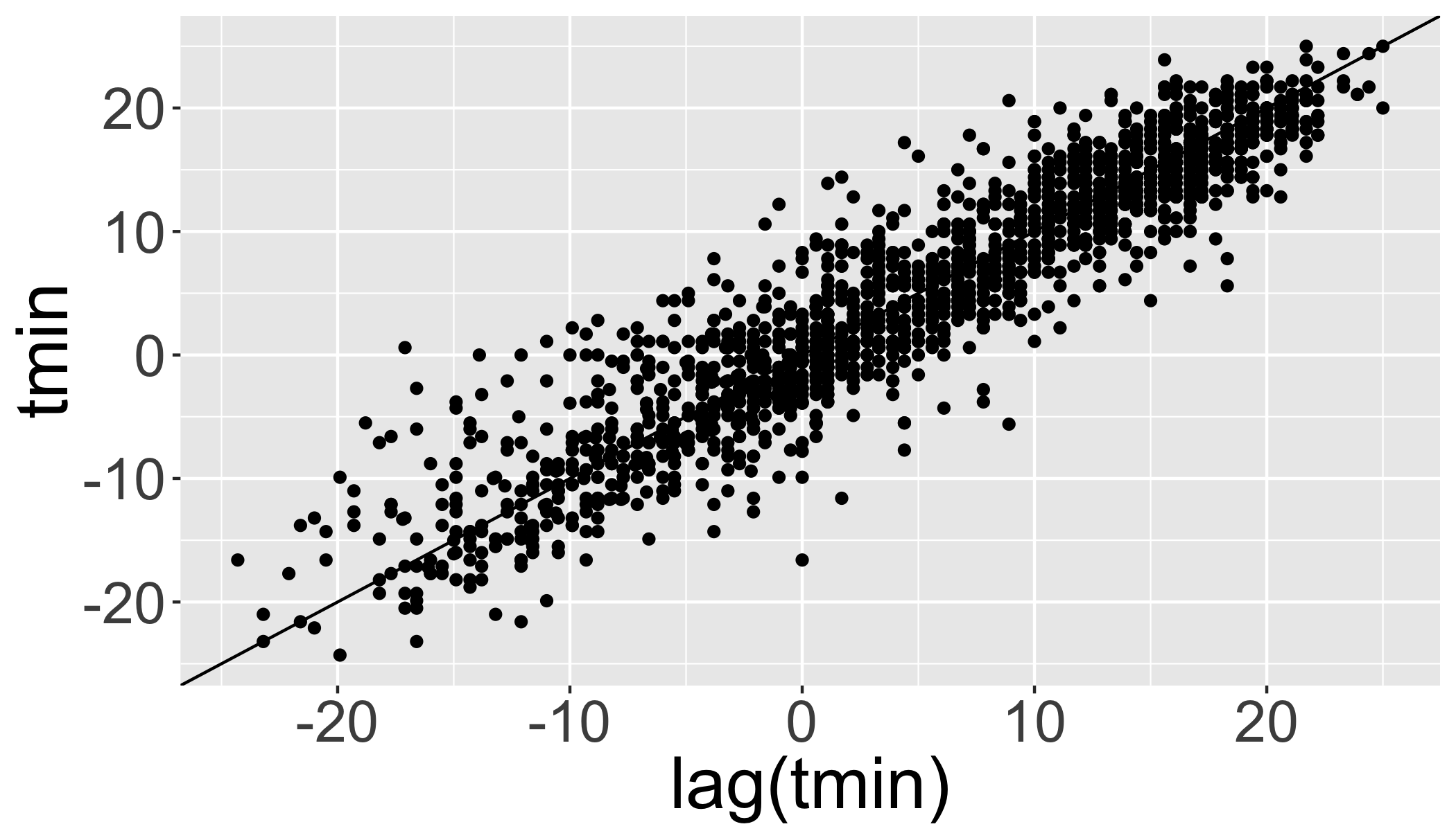

Autocorrelation functions

autocorrelation x vs. x_t − 1 (lag=1)
partial autocorrelation. x vs. x_n after controlling for correlations ∈ t − 1 : n

Autocorrelation

acf(tmin.ts,lag.max = 365*3,na.action = na.exclude )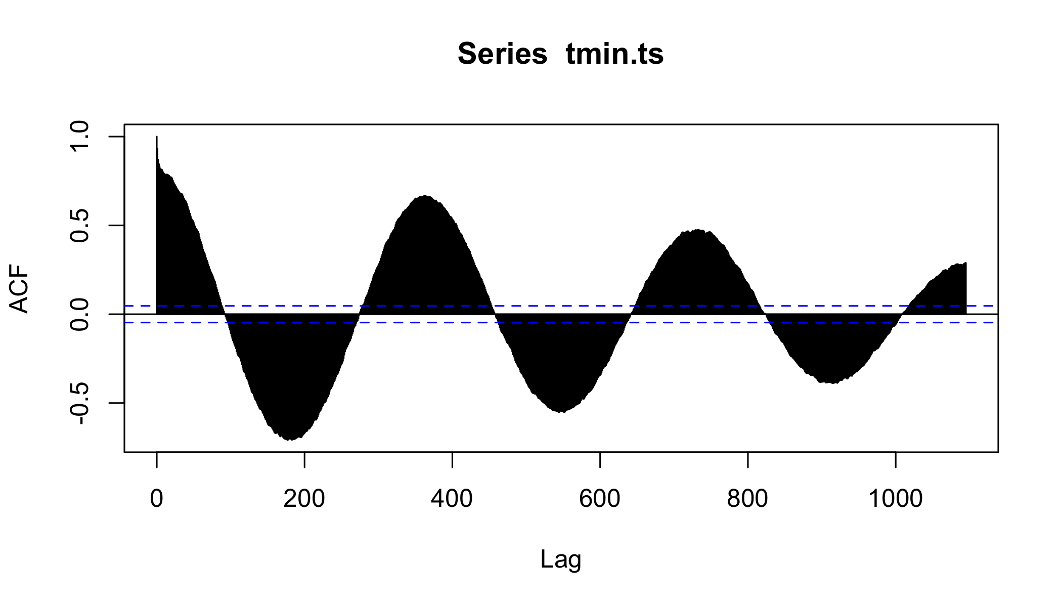

Partial Autocorrelation

pacf(tmin.ts,lag.max = 365*3,na.action = na.exclude )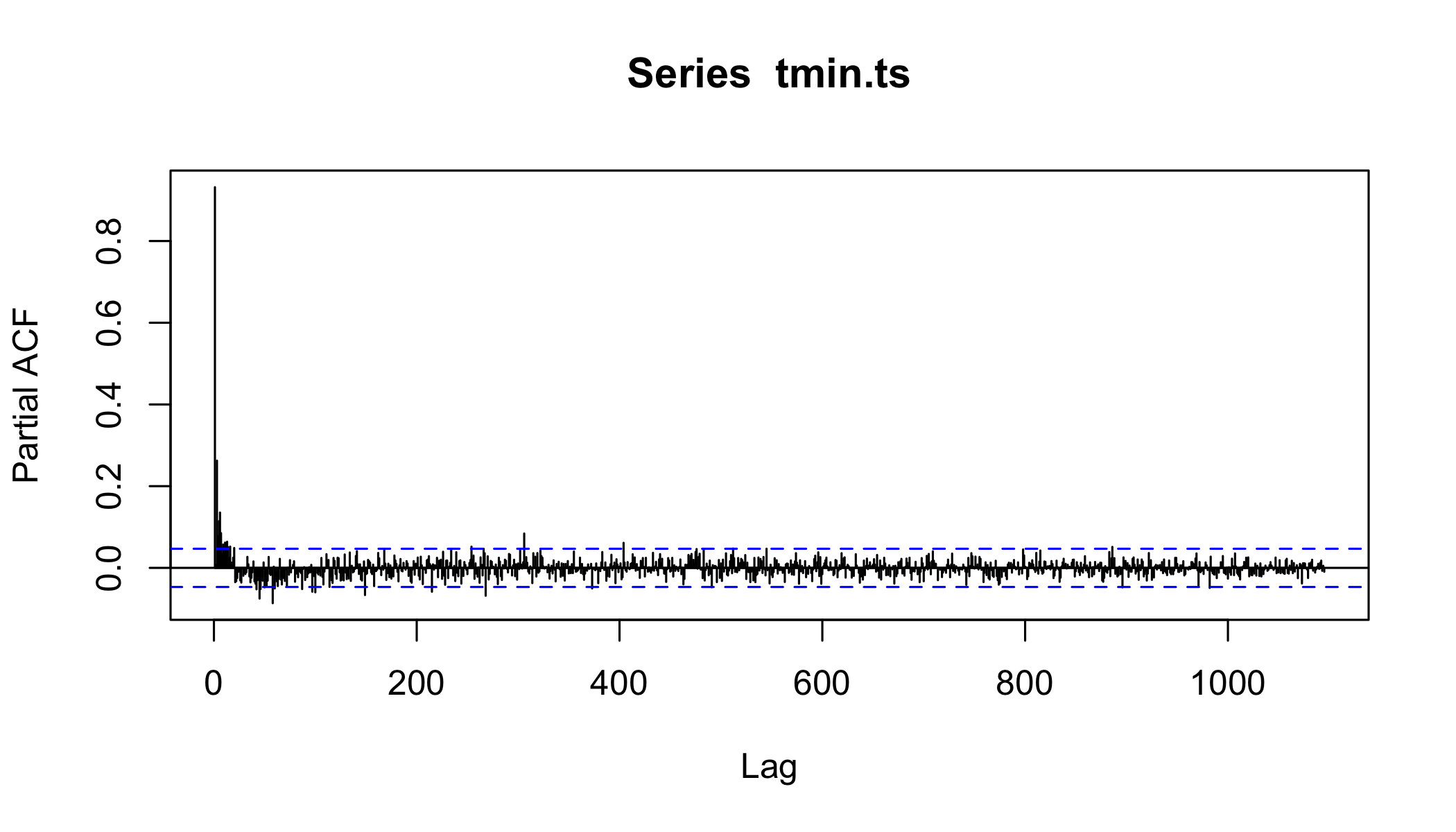

Checking for significant trends

Compute temporal aggregation indices

Group by month, season, year, and decade.

How to convert years into ‘decades’?

## [1] 1938

round(1938,-1)

## [1] 1940

floor(1938/10)*10

## [1] 1930

Calculate seasonal and decadal mean temperatures.

d_filtered2=d_filtered%>%
  mutate(month=as.numeric(format(date,"%m")),
        year=as.numeric(format(date,"%Y")),
        season=ifelse(month%in%c(12,1,2),"Winter",
            ifelse(month%in%c(3,4,5),"Spring",
              ifelse(month%in%c(6,7,8),"Summer",
                ifelse(month%in%c(9,10,11),"Fall",NA)))),
        dec=(floor(as.numeric(format(date,"%Y"))/10)*10))
knitr::kable(head(d_filtered2))

id	date	mflag_prcp	prcp	tmax	tmin	month	year	season	dec
USW00014733	1938-05-01	T	0	14.4	3.9	5	1938	Spring	1930
USW00014733	1938-05-02	T	0	21.1	8.3	5	1938	Spring	1930
USW00014733	1938-05-03		25	16.7	7.2	5	1938	Spring	1930
USW00014733	1938-05-04		112	20.6	9.4	5	1938	Spring	1930
USW00014733	1938-05-05	T	0	31.1	10.6	5	1938	Spring	1930
USW00014733	1938-05-06		64	19.4	7.8	5	1938	Spring	1930

Timeseries models

How to assess change? Simple differences?

d_filtered2%>%
  mutate(period=ifelse(year<=1976-01-01,"early","late"))%>% #create two time periods before and after 1976
  group_by(period)%>%  # divide the data into the two groups
  summarize(n=n(),    # calculate the means between the two periods
            tmin=mean(tmin,na.rm=T),
            tmax=mean(tmax,na.rm=T),
            prcp=mean(prcp,na.rm=T))

## # A tibble: 2 x 5
##   period     n  tmin  tmax  prcp
##   <chr>  <int> <dbl> <dbl> <dbl>
## 1 early  13394  4.20  13.7  25.1
## 2 late   15645  4.76  13.8  28.4

But be careful, there were lots of missing data in the beginning of the record

d_filtered2%>%
  group_by(year)%>%
  summarize(n=n())%>%
  ggplot(aes(x=year,y=n))+
  geom_line(col="grey")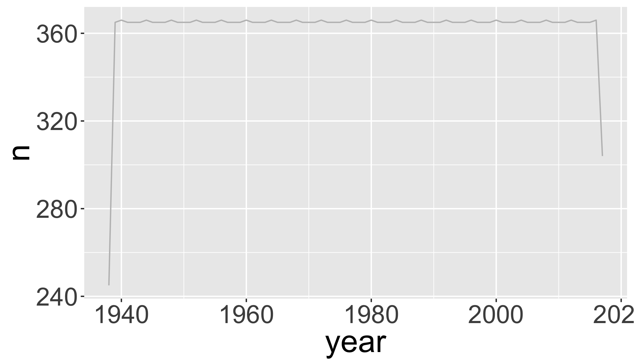

# which years don't have complete data?
d_filtered2%>%
  group_by(year)%>%
  summarize(n=n())%>%
  filter(n<360)

## # A tibble: 2 x 2
##    year     n
##   <dbl> <int>
## 1  1938   245
## 2  2017   304

Plot 10-year means (excluding years without complete data):

d_filtered2%>%
  filter(year>1938, year<2017)%>%
  group_by(dec)%>%
  summarize(
            n=n(),
            tmin=mean(tmin,na.rm=T),
            tmax=mean(tmax,na.rm=T),
            prcp=mean(prcp,na.rm=T)
            )%>%
  ggplot(aes(x=dec,y=tmax))+
  geom_line(col="grey")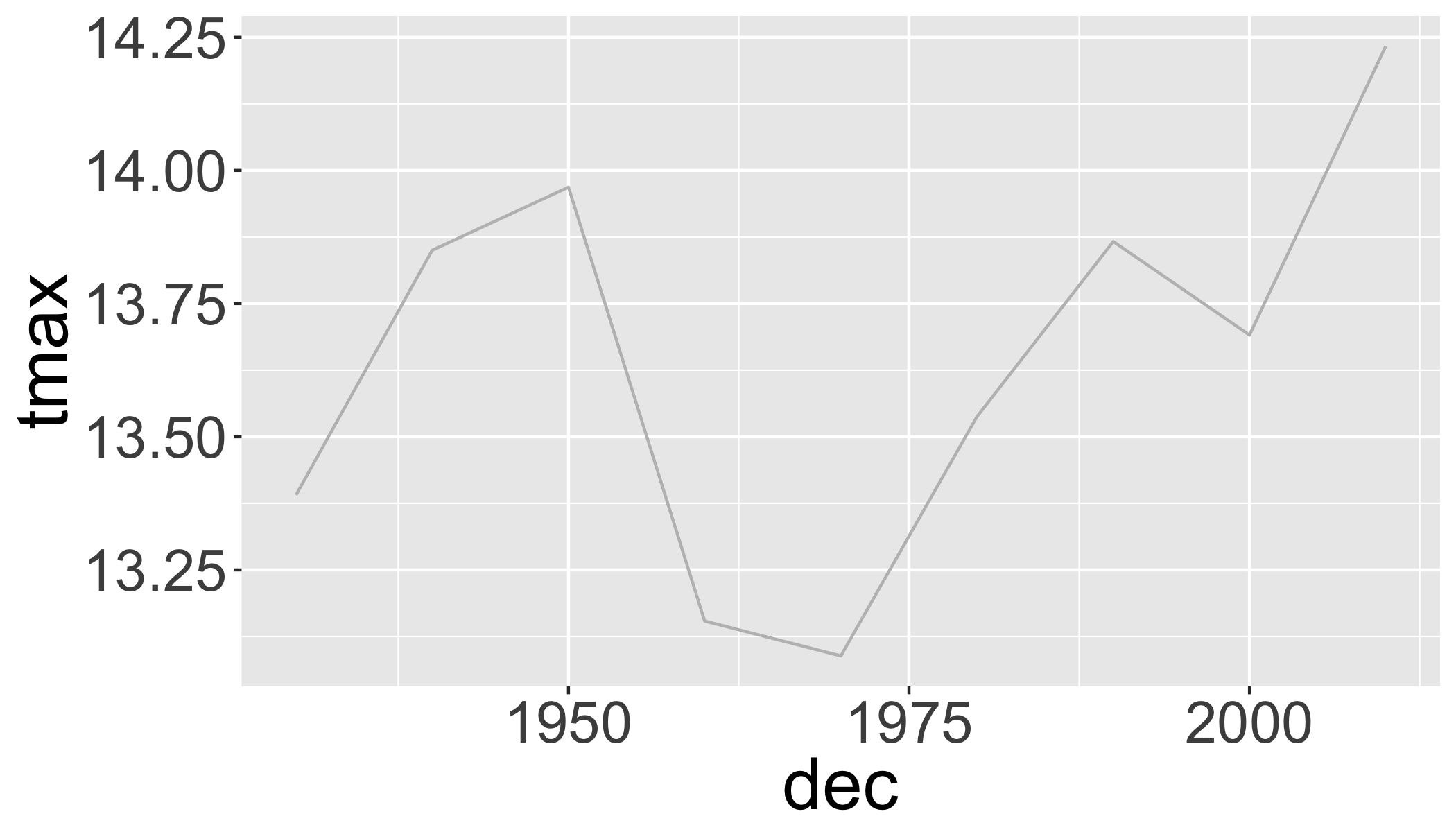

Look for specific events: was 2017 unusually hot in Buffalo, NY?

Let’s compare 2017 with all the previous years in the dataset. First add ‘day of year’ to the data to facilitate showing all years on the same plot.

df=d_filtered2%>%
  mutate(doy=as.numeric(format(date,"%j")),
         doydate=as.Date(paste("2017-",doy),format="%Y-%j"))

Then plot all years (in grey) and add 2017 in red.

ggplot(df,aes(x=doydate,y=tmax,group=year))+
  geom_line(col="grey",alpha=.5)+ # plot each year in grey
  stat_smooth(aes(group=1),col="black")+   # Add a smooth GAM to estimate the long-term mean
  geom_line(data=filter(df,year>2016),col="red")+  # add 2017 in red
  scale_x_date(labels = date_format("%b"),date_breaks = "2 months")

## `geom_smooth()` using method = 'gam' and formula 'y ~ s(x, bs = "cs")'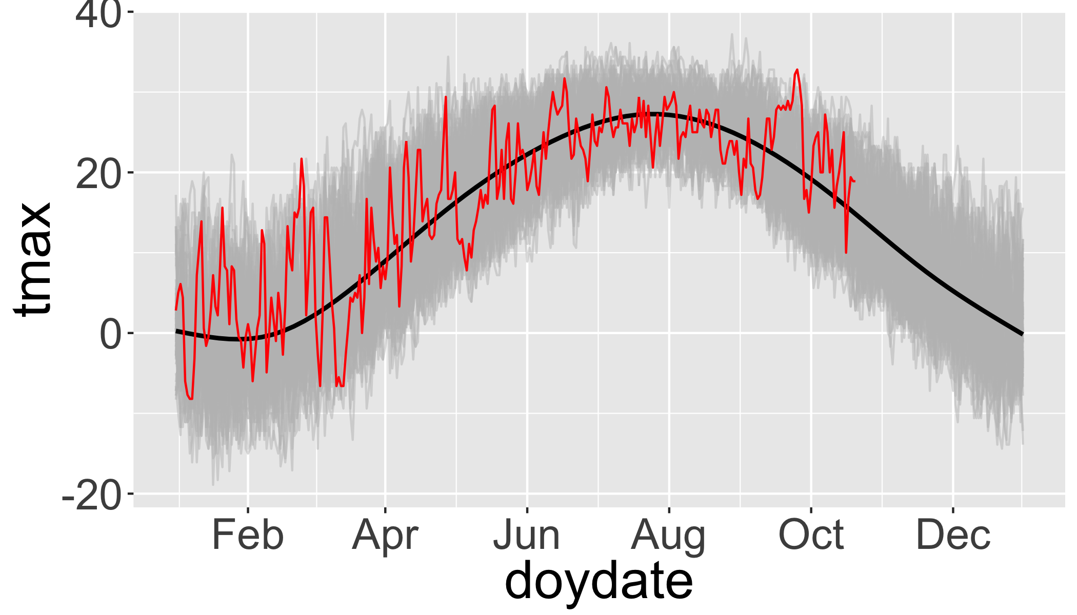

Then ‘zoom’ into just the past few months and add 2017 in red.

ggplot(df,aes(x=doydate,y=tmax,group=year))+
  geom_line(col="grey",alpha=.5)+
  stat_smooth(aes(group=1),col="black")+
  geom_line(data=filter(df,year>2016),col="red")+
  scale_x_date(labels = date_format("%b"),date_breaks = "2 months",
               lim=c(as.Date("2017-08-01"),as.Date("2017-10-31")))

## `geom_smooth()` using method = 'gam' and formula 'y ~ s(x, bs = "cs")'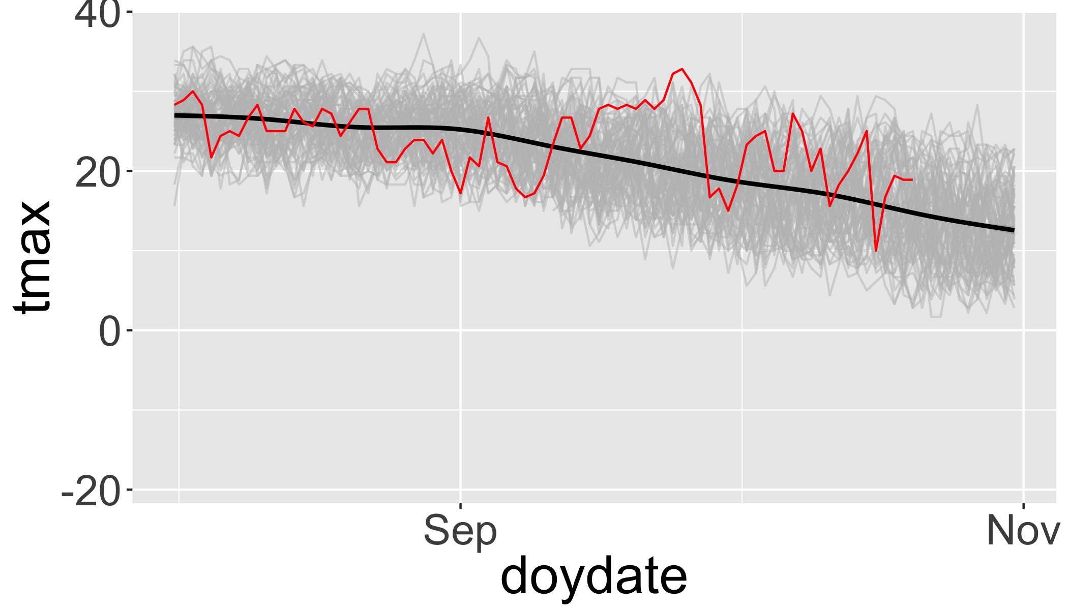

So there was an unusually warm spell in late September.

Summarize by season

seasonal=d_filtered2%>%
  group_by(year,season)%>%
  summarize(n=n(),
            tmin=mean(tmin),
            tmax=mean(tmax),
            prcp=mean(prcp))%>%
  filter(n>75)

ggplot(seasonal,aes(y=tmin,x=year))+
  facet_grid(season~.,scales = "free_y")+
  stat_smooth(method="lm", se=T)+
  geom_line()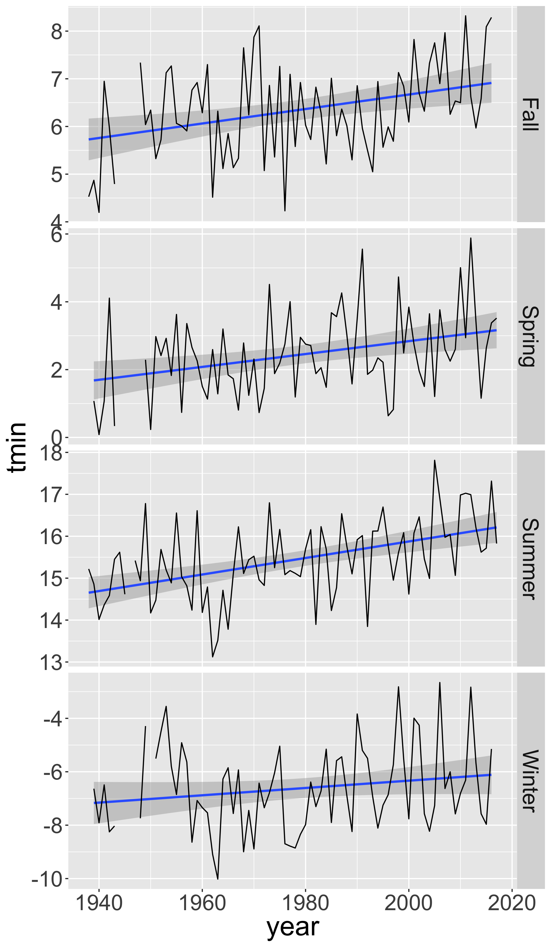

Linear regression of maximum temperature in fall

s1=seasonal%>%
  filter(season=="Summer")

ggplot(s1,aes(y=tmin,x=year))+
  stat_smooth(method="lm", se=T)+
  geom_line()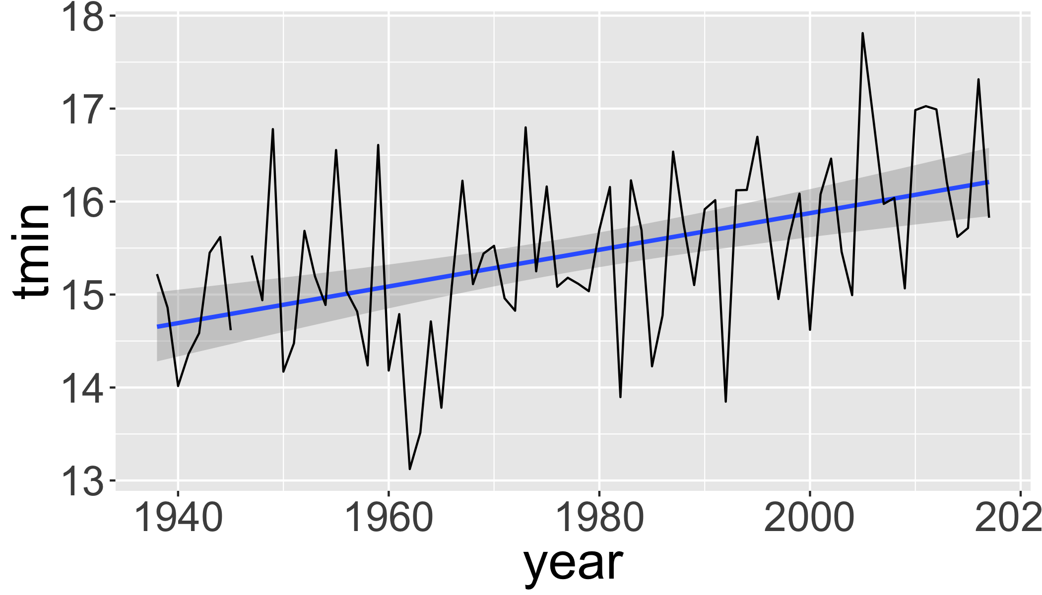

lm1=lm(tmin~year, data=s1)
str(lm1)

## List of 13
##  $ coefficients : Named num [1:2] -23.551 0.0197
##   ..- attr(*, "names")= chr [1:2] "(Intercept)" "year"
##  $ residuals    : Named num [1:79] 0.566 0.187 -0.676 -0.349 -0.147 ...
##   ..- attr(*, "names")= chr [1:79] "1" "2" "3" "4" ...
##  $ effects      : Named num [1:79] -137.232 4.023 -0.752 -0.424 -0.222 ...
##   ..- attr(*, "names")= chr [1:79] "(Intercept)" "year" "" "" ...
##  $ rank         : int 2
##  $ fitted.values: Named num [1:79] 14.7 14.7 14.7 14.7 14.7 ...
##   ..- attr(*, "names")= chr [1:79] "1" "2" "3" "4" ...
##  $ assign       : int [1:2] 0 1
##  $ qr           :List of 5
##   ..$ qr   : num [1:79, 1:2] -8.888 0.113 0.113 0.113 0.113 ...
##   .. ..- attr(*, "dimnames")=List of 2
##   .. .. ..$ : chr [1:79] "1" "2" "3" "4" ...
##   .. .. ..$ : chr [1:2] "(Intercept)" "year"
##   .. ..- attr(*, "assign")= int [1:2] 0 1
##   ..$ qraux: num [1:2] 1.11 1.17
##   ..$ pivot: int [1:2] 1 2
##   ..$ tol  : num 1e-07
##   ..$ rank : int 2
##   ..- attr(*, "class")= chr "qr"
##  $ df.residual  : int 77
##  $ na.action    :Class 'omit'  Named int 9
##   .. ..- attr(*, "names")= chr "9"
##  $ xlevels      : Named list()
##  $ call         : language lm(formula = tmin ~ year, data = s1)
##  $ terms        :Classes 'terms', 'formula'  language tmin ~ year
##   .. ..- attr(*, "variables")= language list(tmin, year)
##   .. ..- attr(*, "factors")= int [1:2, 1] 0 1
##   .. .. ..- attr(*, "dimnames")=List of 2
##   .. .. .. ..$ : chr [1:2] "tmin" "year"
##   .. .. .. ..$ : chr "year"
##   .. ..- attr(*, "term.labels")= chr "year"
##   .. ..- attr(*, "order")= int 1
##   .. ..- attr(*, "intercept")= int 1
##   .. ..- attr(*, "response")= int 1
##   .. ..- attr(*, ".Environment")=<environment: R_GlobalEnv> 
##   .. ..- attr(*, "predvars")= language list(tmin, year)
##   .. ..- attr(*, "dataClasses")= Named chr [1:2] "numeric" "numeric"
##   .. .. ..- attr(*, "names")= chr [1:2] "tmin" "year"
##  $ model        :'data.frame':   79 obs. of  2 variables:
##   ..$ tmin: num [1:79] 15.2 14.9 14 14.4 14.6 ...
##   ..$ year: num [1:79] 1938 1939 1940 1941 1942 ...
##   ..- attr(*, "terms")=Classes 'terms', 'formula'  language tmin ~ year
##   .. .. ..- attr(*, "variables")= language list(tmin, year)
##   .. .. ..- attr(*, "factors")= int [1:2, 1] 0 1
##   .. .. .. ..- attr(*, "dimnames")=List of 2
##   .. .. .. .. ..$ : chr [1:2] "tmin" "year"
##   .. .. .. .. ..$ : chr "year"
##   .. .. ..- attr(*, "term.labels")= chr "year"
##   .. .. ..- attr(*, "order")= int 1
##   .. .. ..- attr(*, "intercept")= int 1
##   .. .. ..- attr(*, "response")= int 1
##   .. .. ..- attr(*, ".Environment")=<environment: R_GlobalEnv> 
##   .. .. ..- attr(*, "predvars")= language list(tmin, year)
##   .. .. ..- attr(*, "dataClasses")= Named chr [1:2] "numeric" "numeric"
##   .. .. .. ..- attr(*, "names")= chr [1:2] "tmin" "year"
##   ..- attr(*, "na.action")=Class 'omit'  Named int 9
##   .. .. ..- attr(*, "names")= chr "9"
##  - attr(*, "class")= chr "lm"

summary(lm1)

## 
## Call:
## lm(formula = tmin ~ year, data = s1)
## 
## Residuals:
##      Min       1Q   Median       3Q      Max 
## -2.00360 -0.45550 -0.02385  0.57754  1.90919 
## 
## Coefficients:
##               Estimate Std. Error t value Pr(>|t|)    
## (Intercept) -23.551009   8.042522  -2.928  0.00448 ** 
## year          0.019713   0.004066   4.848 6.33e-06 ***
## ---
## Signif. codes:  0 '***' 0.001 '**' 0.01 '*' 0.05 '.' 0.1 ' ' 1
## 
## Residual standard error: 0.8298 on 77 degrees of freedom
##   (1 observation deleted due to missingness)
## Multiple R-squared:  0.2339, Adjusted R-squared:  0.2239 
## F-statistic: 23.51 on 1 and 77 DF,  p-value: 6.333e-06

You can extract values of interest by looking at the structure of the object.

str(summary(lm1))

## List of 12
##  $ call         : language lm(formula = tmin ~ year, data = s1)
##  $ terms        :Classes 'terms', 'formula'  language tmin ~ year
##   .. ..- attr(*, "variables")= language list(tmin, year)
##   .. ..- attr(*, "factors")= int [1:2, 1] 0 1
##   .. .. ..- attr(*, "dimnames")=List of 2
##   .. .. .. ..$ : chr [1:2] "tmin" "year"
##   .. .. .. ..$ : chr "year"
##   .. ..- attr(*, "term.labels")= chr "year"
##   .. ..- attr(*, "order")= int 1
##   .. ..- attr(*, "intercept")= int 1
##   .. ..- attr(*, "response")= int 1
##   .. ..- attr(*, ".Environment")=<environment: R_GlobalEnv> 
##   .. ..- attr(*, "predvars")= language list(tmin, year)
##   .. ..- attr(*, "dataClasses")= Named chr [1:2] "numeric" "numeric"
##   .. .. ..- attr(*, "names")= chr [1:2] "tmin" "year"
##  $ residuals    : Named num [1:79] 0.566 0.187 -0.676 -0.349 -0.147 ...
##   ..- attr(*, "names")= chr [1:79] "1" "2" "3" "4" ...
##  $ coefficients : num [1:2, 1:4] -23.55101 0.01971 8.04252 0.00407 -2.92831 ...
##   ..- attr(*, "dimnames")=List of 2
##   .. ..$ : chr [1:2] "(Intercept)" "year"
##   .. ..$ : chr [1:4] "Estimate" "Std. Error" "t value" "Pr(>|t|)"
##  $ aliased      : Named logi [1:2] FALSE FALSE
##   ..- attr(*, "names")= chr [1:2] "(Intercept)" "year"
##  $ sigma        : num 0.83
##  $ df           : int [1:3] 2 77 2
##  $ r.squared    : num 0.234
##  $ adj.r.squared: num 0.224
##  $ fstatistic   : Named num [1:3] 23.5 1 77
##   ..- attr(*, "names")= chr [1:3] "value" "numdf" "dendf"
##  $ cov.unscaled : num [1:2, 1:2] 93.928528 -0.047483 -0.047483 0.000024
##   ..- attr(*, "dimnames")=List of 2
##   .. ..$ : chr [1:2] "(Intercept)" "year"
##   .. ..$ : chr [1:2] "(Intercept)" "year"
##  $ na.action    :Class 'omit'  Named int 9
##   .. ..- attr(*, "names")= chr "9"
##  - attr(*, "class")= chr "summary.lm"

summary(lm1)$r.squared

## [1] 0.2338852

Print a summary table:

tidy(lm1)

## # A tibble: 2 x 5
##   term        estimate std.error statistic    p.value
##   <chr>          <dbl>     <dbl>     <dbl>      <dbl>
## 1 (Intercept) -23.6      8.04        -2.93 0.00448   
## 2 year          0.0197   0.00407      4.85 0.00000633

Autoregressive models

See Time Series Analysis Task View for summary of available packages/models.

Moving average (MA) models
autoregressive (AR) models
autoregressive moving average (ARMA) models
frequency analysis
Many, many more…

Climate Metrics

Climdex indices

ClimDex

Format data for `climdex`

library(PCICt)
## Parse the dates into PCICt.
pc.dates <- as.PCICt(as.POSIXct(d_filtered$date),cal="gregorian")

Generate the climdex object

  library(climdex.pcic)
    ci <- climdexInput.raw(
      tmax=d_filtered$tmax,
      tmin=d_filtered$tmin,
      prec=d_filtered$prcp,
      pc.dates,pc.dates,pc.dates, 
      base.range=c(1971, 2000))
years=as.numeric(as.character(unique(ci@date.factors$annual)))

Cumulative dry days

cdd= climdex.cdd(ci, spells.can.span.years = TRUE)
plot(cdd~years,type="l")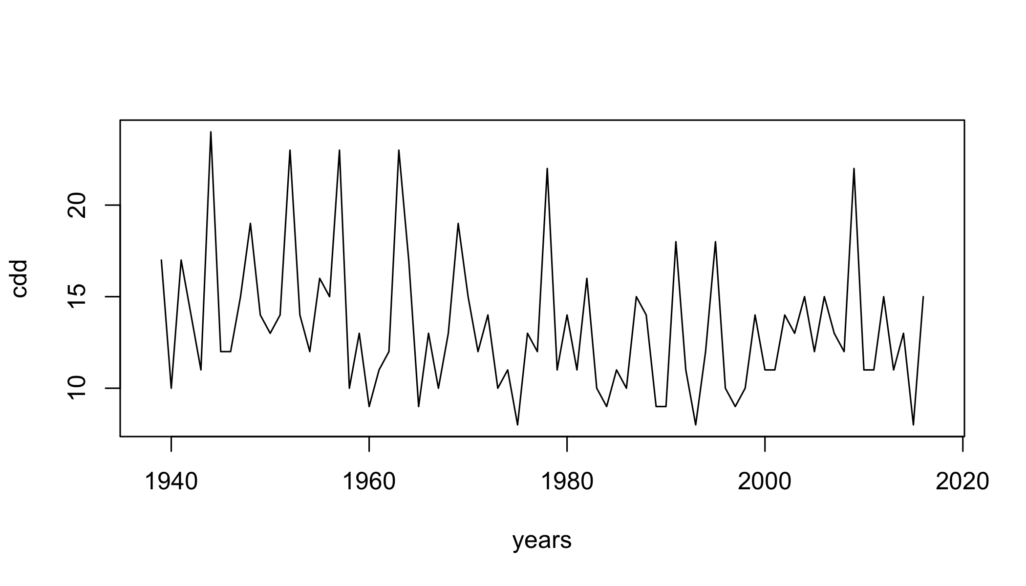

Diurnal Temperature Range

dtr=climdex.dtr(ci, freq = c("annual"))
plot(dtr~years,type="l")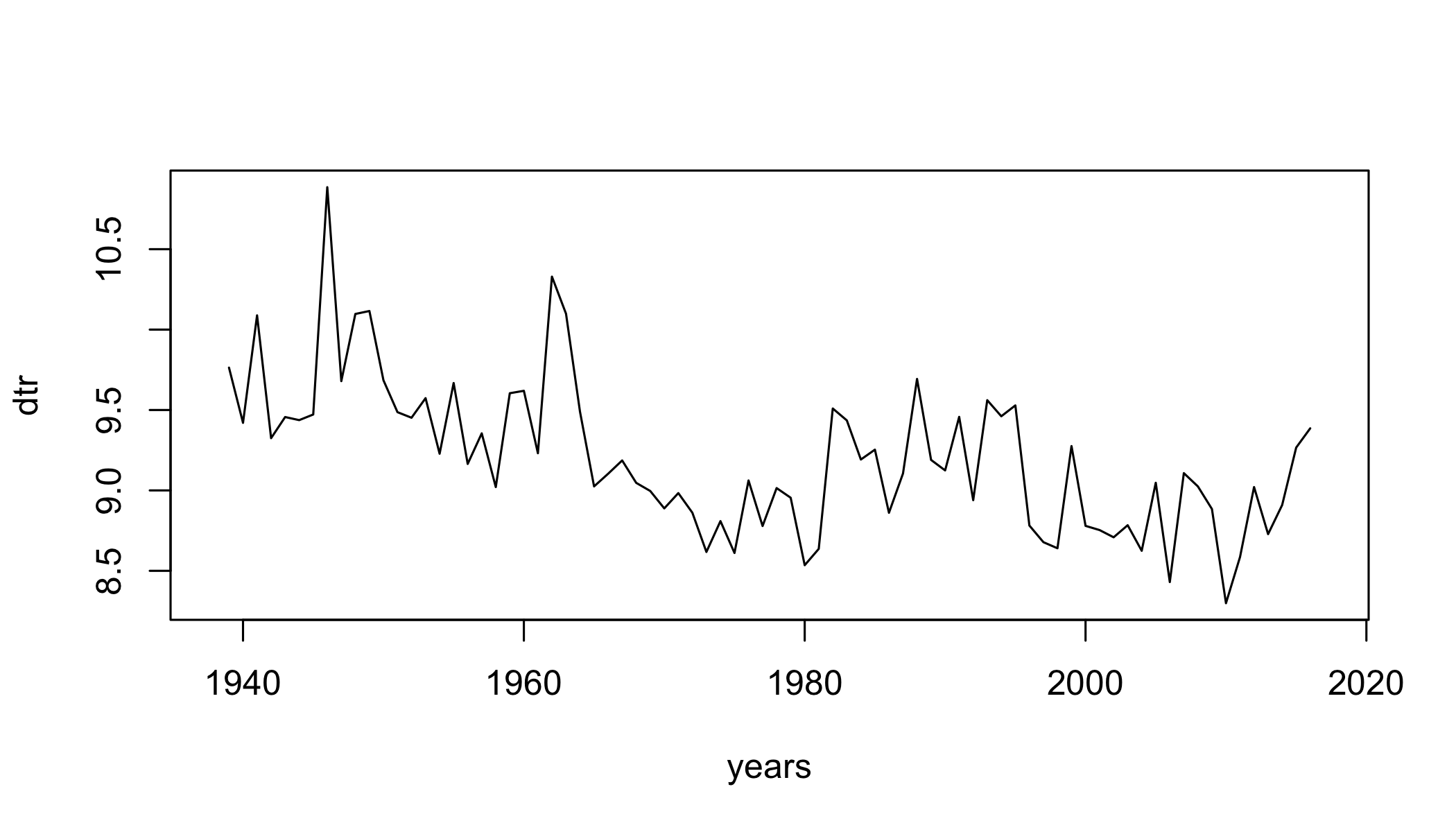

Frost Days

fd=climdex.fd(ci)
plot(fd~years,type="l")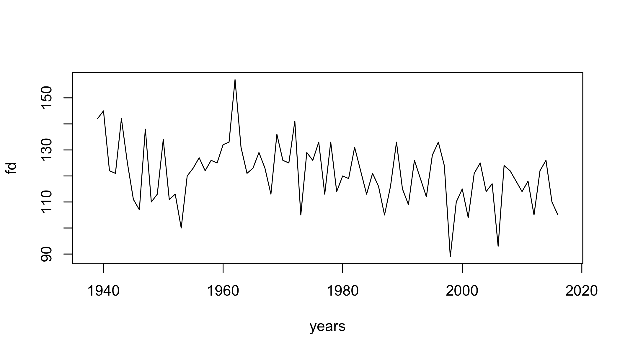

Your Turn

See all available indices with:

climdex.get.available.indices(ci)

##  [1] "climdex.su"      "climdex.id"      "climdex.txx"    
##  [4] "climdex.txn"     "climdex.tx10p"   "climdex.tx90p"  
##  [7] "climdex.wsdi"    "climdex.fd"      "climdex.tr"     
## [10] "climdex.tnx"     "climdex.tnn"     "climdex.tn10p"  
## [13] "climdex.tn90p"   "climdex.csdi"    "climdex.rx1day" 
## [16] "climdex.rx5day"  "climdex.sdii"    "climdex.r10mm"  
## [19] "climdex.r20mm"   "climdex.rnnmm"   "climdex.cdd"    
## [22] "climdex.cwd"     "climdex.r95ptot" "climdex.r99ptot"
## [25] "climdex.prcptot" "climdex.gsl"     "climdex.dtr"

Select 3 indices, calculate them, and plot the timeseries.

r10mm=climdex.r10mm(ci)
plot(r10mm~years,type="l")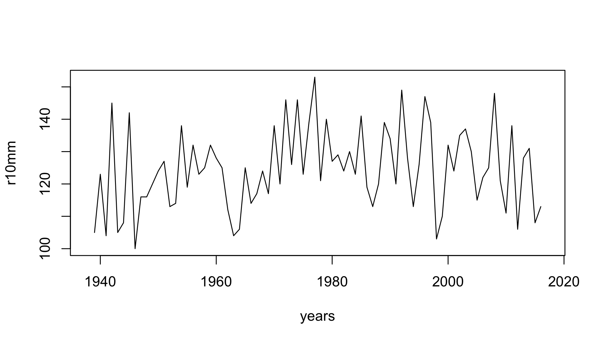

prcptot=climdex.prcptot(ci)
plot(prcptot~years,type="l")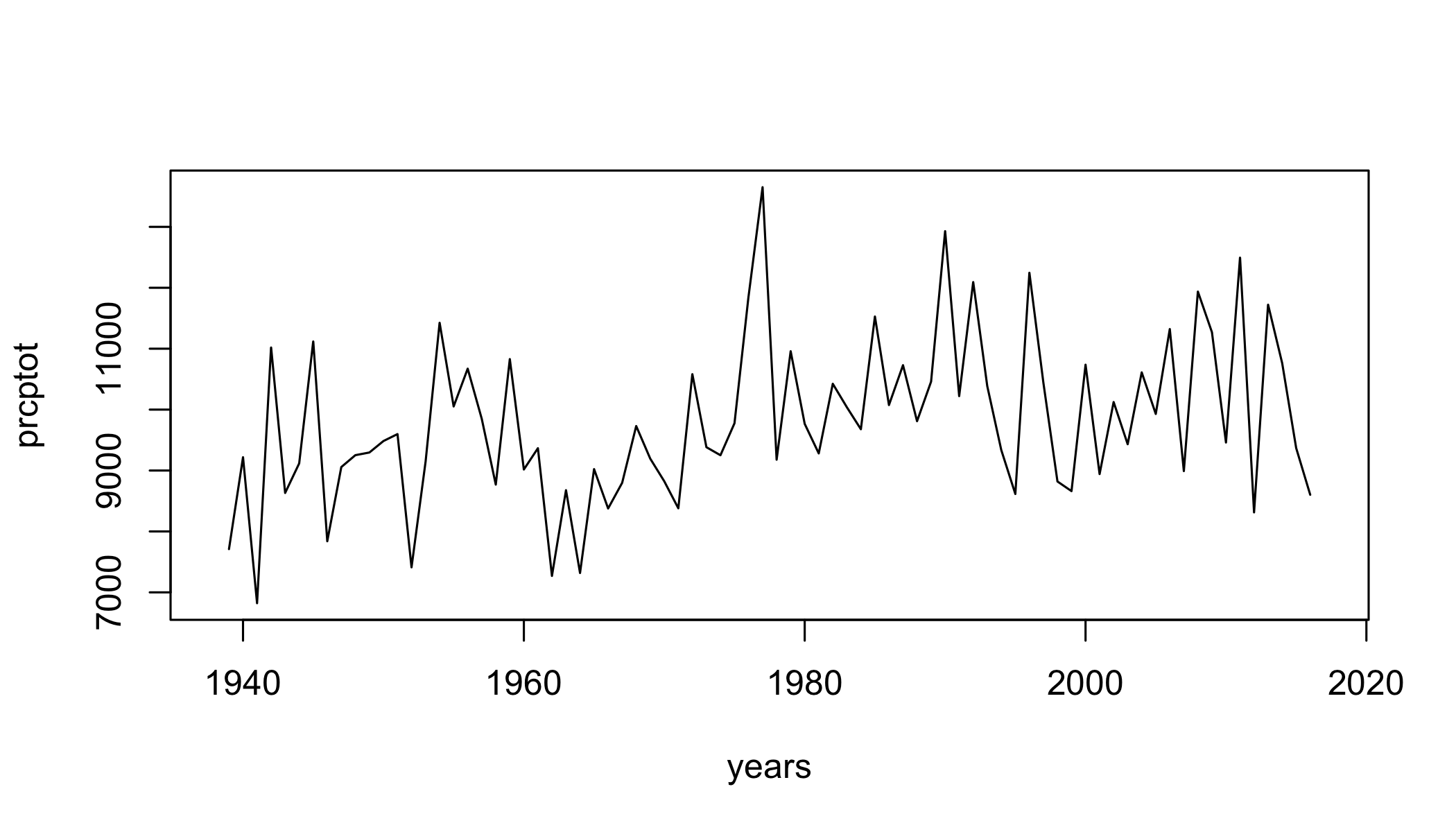

gsl=climdex.gsl(ci)
plot(gsl~years,type="l")

Climate Metrics from daily weather data

Summary

Climate Metrics

Climate Metrics: ClimdEX

27 Core indices

Weather Data

Climate Data Online

GHCN

Options for downloading data

FedData package

NOAA API

rNOAA package

Libraries

Station locations

GHCND Variables

filter() to temperature and precipitation

Map GHCND stations

Your turn

Download daily data from GHCN

geocode in ggmap package useful for geocoding place names

Quality Control: MFLAG

Quality Control: QFLAG

Quality Control: SFLAG

Summarize QC flags

Filter with QC data and change units

Zoo package for rolling functions

Your Turn

Time Series analysis

Temporal autocorrelation

Autocorrelation functions

Autocorrelation

Partial Autocorrelation

Checking for significant trends

Compute temporal aggregation indices

Group by month, season, year, and decade.

Timeseries models

Look for specific events: was 2017 unusually hot in Buffalo, NY?

Summarize by season

Linear regression of maximum temperature in fall

Autoregressive models

Climate Metrics

Climdex indices

Format data for climdex

Generate the climdex object

Cumulative dry days

Diurnal Temperature Range

Frost Days

Your Turn

`FedData` package

`rNOAA` package

`filter()` to temperature and precipitation

`geocode` in ggmap package useful for geocoding place names

Format data for `climdex`